Preface
A heartbeat on the skin is about a millivolt. A brain rhythm on the scalp is a few tens of microvolts. A single neuron, seen from an electrode a few tens of micrometres away, is a hundred microvolts that lasts a millisecond. Every wearable ECG patch, EEG headset, prosthetic-control armband and neural implant has to turn these signals into clean numbers while the patient’s body picks up volts of mains interference, the electrodes add hundreds of millivolts of offset, and the battery allows a few microwatts per channel. The chip that does this is a biopotential analog front-end (AFE) and its data converters.
This tutorial teaches you to design one by following a single, concrete chip, Open-BioAFE: an 8-channel ECG/EEG/EMG front-end with a 12-bit SAR and a 16-bit incremental ΔΣ converter, built in the open-source IHP SG13G2 130 nm SiGe BiCMOS process [1] with open-source tools [2]. Every concept follows the same pattern as our Open-SERDES tutorial [3]: a short derivation, a worked example with the project’s real numbers, and a what this means for your design box.
Who this tutorial is for. Third- and fourth-year electrical engineering undergraduates and first-year graduate students, and biomedical engineers who need to specify the hardware they will use. After reading it you should be able to:
- turn a clinical or research application into a front-end specification: channels, bandwidth, noise, CMRR, input impedance, offset range and power;
- design and budget a low-noise, low-power amplifier chain: chopping, DC servo loops, filters and right-leg drive;
- choose, size and verify a SAR or ΔΣ converter for a biosignal;
- show, with real ECG, EEG and EMG recordings, how the circuit choices move a clinical result;
- carry a block from schematic to a verified layout with open tools, ready for an IHP OpenMPW shuttle.
Prerequisites. Circuit analysis, signals and systems (Fourier and Laplace transforms, filters) and one course in analog electronics (small-signal MOS and BJT models, the differential pair, op-amps), plus some Python. The transistor-level background of Part II, in particular the \(g_\mathrm{m}/I_\mathrm{D}\) method, is taught in Part II of The Art of Analog IC Design [4]; we cross-link it instead of repeating it.
How the tutorial is organised
The tutorial has six parts and a section of hands-on labs. Part I, Foundations (Chapters 1–4), explains where biopotentials come from, what the electrodes and the body do to them, and the interference, safety rules and standards every front-end must meet. Part II, The Analog Front-End (Chapters 5–12), designs the low-noise, low-power amplifier chain. Part III, Data Converters (Chapters 13–22), is the heart of the tutorial: it takes you from the quantiser to a measured SAR and ΔΣ converter. Part IV, Biosignal Processing and Systems (Chapters 23–28), processes real ECG, EEG and EMG data, puts processing on chip and adds bioimpedance sensing. Part V, Putting It Together (Chapters 29–30), assembles the architecture and its budgets and walks through the open-source flow. Part VI, Wearable Systems (Chapters 31–33), takes the chip onto a moving person: signal quality and motion artefacts, ear-EEG and multimodal sensing at the ear, and closed-loop systems. The fifteen Hands-On Labs and their capstone follow the parts, each lab on its own page.
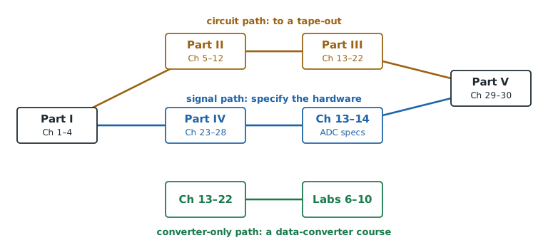
Three reading paths. Everyone should read Part I first. After that, Figure P.1 suggests three routes. The circuit path (Parts I, II, III and V) is for students heading to a tape-out. The signal path (Part I, Part IV, the converter specifications of Chapters 13 and 14, then Part V) is for biomedical-engineering and DSP students who need to specify, not build, the hardware. The converter-only path (Chapter 13 to Chapter 22 with Labs 6–10) is a self-contained course on data converters.
How to read the boxes
Chapters open with what you will learn and close with key takeaways. In between, six kinds of boxes mark the role of each piece of text:
A 20 µV rms EEG rhythm over the 1.5 µVrms noise target of Open-BioAFE gives \(\mathrm{SNR} = 20\log_{10}(20/1.5) \approx 22.5\ \text{dB}\).
An insight box says what a result means for the Open-BioAFE design.
A pitfall box warns about a common mistake, such as quoting an amplitude in rms when the specification is peak-to-peak.
A try-it box points to a lab script (Lab 1).
A specnote box states an Open-BioAFE target: input-referred noise below 1.5 µVrms from 0.5 to 100 Hz in EEG mode.
Longer algebra sits in grey derivation boxes.
How the labs work
Fifteen labs in three tracks use only free tools: Python (NumPy, SciPy, wfdb, python-deltasigma) for signals and system models, Xschem and ngspice for transistor-level SG13G2 circuits, and KLayout for layout (Hands-On Labs). The Python labs live in labs/python/ and share one module, biosig.py, which holds the signal tables, the synthetic signals and the electrode and interference models. The figure scripts in figsrc/ import the same module, so the numbers on these pages and the numbers your labs print come from the same code. Datasets stay on PhysioNet [5] and NinaPro [6] under their own licences; the labs download them on first use.
The state of this draft
This is release v0.1 (November 2026). All thirty-three chapters, the five appendices and the fifteen hands-on labs are written; the SG13G2 labs have scripts that run in the IIC-OSIC-TOOLS container, the real-data labs read PhysioNet recordings, and most chapters carry an interactive demo. Expect corrections as the labs are run on silicon.
Sources and acknowledgments
The biomedical-instrumentation chapters draw on Webster’s Medical Instrumentation [7] and on Yazicioglu, Van Hoof and Puers’ Biopotential Readout Circuits [8]; the converter chapters on Pelgrom [9] and on Schreier, Temes and Pavan [10]. The chip is possible because IHP opened its SG13G2 process design kit [1] and the Institute for Integrated Circuits at JKU Linz maintains the IIC-OSIC-TOOLS container and the analog chip template [2, 11]. The labs use open data from PhysioNet [5] and NinaPro [6].
This is a living draft (v0.1); numbers will be refined as the design matures. If you find an error, an unclear derivation or a figure that does not explain what it should, please email bricd.org@gmail.com or open an issue or a pull request on the project’s GitHub repository, linked from thebricd.org.
How this tutorial was made
This tutorial, its figures and its lab code were developed with the help of AI tools, and this draft may contain mistakes; please report any you find as described above, and we will correct them. The topics, structure and many of the results follow the sources acknowledged above and listed in the References. Standards are summarised, never reproduced: always work from the edition of IEC 60601 that applies to your device.