Chapter 25EEG Processing and Brain–Computer Interfaces
EEG carries information in rhythms and their changes; most of the processing estimates power in frequency bands.
- compute band power and spectral features;
- choose the segment length and averaging of a spectrum, and predict its scatter;
- remove EOG and EMG artefacts, including with ICA;
- detect seizure onset on the CHB-MIT database;
- explain the basics of SSVEP and motor-imagery BCIs;
- size the integration time of a steady-state detector and the data rate of a feature stream.
Which EEG features need which resolution and sample rate, and what does that save on chip?
The EEG is the most demanding signal of the chip: it sets the 1.5 µVrms noise target and, with the electrode offset, the 16-bit converter (Chapter 2). What the applications extract from it, however, is mostly coarse: the power in a few frequency bands, its changes over seconds, and its spatial pattern across electrodes. This chapter asks how much of the front-end’s precision those features actually use, with a synthetic EEG whose seizure-like segments are known exactly; Lab 12 repeats the study on real recordings from CHB-MIT [32].
25.1Band power and spectral features
EEG rhythms fall into bands: delta (0.5–4 Hz), theta (4–8 Hz), alpha (8–13 Hz), beta (13–30 Hz) and gamma (30–100 Hz). The workhorse feature is the power in each band over a window of one to a few seconds, estimated with Welch’s method [63] (averaged FFTs of overlapping, windowed segments) or with a bank of band-pass filters and a squarer, which is cheaper on chip. Ratios between bands, relative power (band power over total power) and the spectral edge (the frequency below which 90 % of the power lies) follow from the same numbers. Time-domain features such as line length, the sum of absolute sample-to-sample differences, are cheaper still, but, as section 25.3 shows, they respond to noise as well as to rhythms.
By Parseval’s theorem, the power spectral density \(S(f)\) integrated over a band equals the mean square of the signal after an ideal band-pass filter, so a filter and squarer compute the same feature as a spectrum:
Here \(\hat S(f_k)\) is the estimated spectrum in bin \(k\), \(\Delta f\) the bin spacing and \(P_\mathrm{total}\) the power over 0.5–100 Hz. Relative power ignores the channel’s gain and the electrode contact, which scale every band alike. The spectral edge \(f_\mathrm{SEF}\) solves \(\int_{0.5\ \text{Hz}}^{f_\mathrm{SEF}} S\,df = 0.9\,P_\mathrm{total}\).
25.2Artefact removal
The eyes and muscles produce larger signals than the brain. Eye movements and blinks (EOG) add slow, large deflections at the frontal electrodes, below about 4 Hz. Muscle activity (EMG) from the jaw, forehead and neck adds broadband noise above about 20 Hz. Three methods deal with them:
- filtering, which removes the out-of-band part but also the EEG in the same band;
- regression against dedicated EOG electrodes, which subtracts a scaled copy of the eye signal;
- independent component analysis (ICA), which unmixes a multichannel recording into statistically independent sources; components that look like blinks or muscle are removed and the rest are mixed back.
ICA needs many channels and offline computation. On chip, the practical approach is to detect artefacts, by amplitude, slope or the DC servo’s offset monitor (Chapter 10), and flag or discard the affected windows rather than repair them. Chapter 31 turns such flags into a signal-quality index.
25.3Seizure-onset detection
An epileptic seizure typically shows as a rhythmic discharge, often in the theta range, with a large amplitude, building up over seconds. Detectors compute features per window, two seconds in this example, and classify each window. The SoC of Verma et al. [25] computed spectral energy features on chip for exactly this purpose, so that only detections, not raw EEG, had to leave the device.
figsrc/ch25_figs.py adds three 10 s rhythmic discharges (3–6 Hz, 60 µV) to two minutes of synthetic EEG (20 µVrms background) and detects them per 2 s window (Figure 25.1). In EEG mode the total gain of 800 maps ±0.625 mV at the electrodes onto the converter (Chapter 11).
- Line length fails: noise inflates it as much as the discharges do, and a threshold on it does no better than always answering “no seizure” (75 % of windows).
- Theta power (3–8 Hz) with a threshold at three times its median reaches 99 % window accuracy with 6–7 bits (an LSB of 19.5 µV at 6 bits), with input noise from 1.5 up to 15 µVrms. With 4 bits it still reaches 92–95 %.
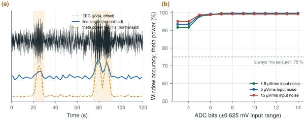
figsrc/ch25_figs.py.Real seizures are less clean than these. On CHB-MIT, patient-specific detectors that combine band powers from several channels perform far better than generic ones, and the useful figures are sensitivity per seizure, detection latency from onset, and false detections per hour. The synthetic study still makes the design point: the detector’s features need far less resolution than the raw recording.
Real EEG can even reverse the ranking. On one hour of a CHB-MIT record (chb01_03, FP1-F7, one seizure), Lab 12 finds the seizure with every detector, but real EEG holds far more theta outside seizures: the theta threshold fires 101 times an hour, line length 12 times. Word length still barely matters down to 6 bits. And even a stationary background crosses a threshold now and then, because a 2 s band power is itself a noisy estimate.
25.4How precise is a band power?
A spectrum estimated from a finite record is random. For a noise-like signal such as the EEG background, each bin of a single periodogram, the squared FFT of one windowed segment, scatters with a standard deviation equal to its mean, 5.6 dB, however long the segment; 4.2 % of bins land more than 5 dB high. A longer segment narrows the bins without steadying them. Welch’s method averages \(K\) shorter segments instead:
The bin spacing depends only on the segment’s duration, not on the sample rate. A Hann window widens each bin to 1.5 bins of noise bandwidth; Hann segments overlapped by half stay nearly independent (16 count as 15.2), and \(K\) of them need \((K+1)\,T_\mathrm{seg}/2\) of record. In decibels the scatter is about \(4.34/\sqrt{K}\). A band power sums every bin of a band of width \(B\), so its scatter depends only on the time–bandwidth product of the whole window \(T\).
The aim: the alpha peak resolved from its neighbours, its height known to ±1 dB.
- Resolution. Ten 0.5 Hz bins across 8–13 Hz need \(T_\mathrm{seg} = 2\) s: 1000 samples at Open-BioAFE’s 500 S/s, 500 at 250 S/s.
- Scatter. One segment gives 5.6 dB (5.55 dB on the synthetic EEG of
biosig.eeg()). For ±1 dB, \(K_\mathrm{eff} \approx 4.34^2 = 19\): 20 overlapping segments, 21 s of recording. Sixteen segments, 17 s, give 1.11 dB (1.17 dB measured, Figure 25.2a); ±0.5 dB takes 81 s. - A band instead of a bin. The alpha-band power of one 2 s epoch averages \(BT = 10\) values: \(1/\sqrt{10} = 32\) %, or 1.37 dB, nearly as steady as one bin after 21 s.
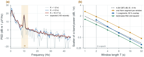
figsrc/ch25_figs.py.The estimator matters too (Figure 25.2b). Over 2 s, one Hann-windowed segment, as in Worked Example 25.1, scatters by 1.91 dB, not 1.37: its taper makes it count as 51 % of its length. Three overlapping 1 s segments give 1.54 dB; a band-pass filter and squarer, weighting every sample equally, 1.15 dB. That sets a false-detection floor: on 20 hours of stationary synthetic background, the theta detector of Worked Example 25.1 fires 12 times an hour with one Hann segment per window, 1.2 times with 1 s segments, and never in 35 400 windows with a filter and squarer.
- Input noise. 1.5 µVrms over 99.5 Hz leaves \(1.5\sqrt{5/99.5} = 0.34\) µVrms in the 5 Hz alpha band. A 10 µVrms rhythm stands 29.5 dB above it, 13 dB better than over the whole band (Chapter 2).
- The brain’s background in the alpha band is 3.2 µVrms in the synthetic EEG, ten times the input noise. The noise adds 0.3 % to theta power, 1.1 % to alpha, 4.2 % to beta and a third to gamma.
- Eight bits over ±0.625 mV (an LSB of 4.88 µV) give 1.41 µVrms of quantisation noise, spread up to 125 Hz at 250 S/s: \(1.41\sqrt{5/125} = 0.28\) µVrms in the alpha band (0.282 µVrms simulated), below the input noise. They add 0.8 % to alpha power and 23 % to gamma.
For scalp EEG the brain’s background, not the front-end, limits alpha and theta band powers; the 1.5 µVrms target matters for gamma, raw recordings and smaller signals such as ear-EEG (Chapter 32). Feed the feature path 8-bit samples at 250 S/s, and use a filter and squarer rather than one windowed FFT per epoch: the estimator, not the converter, sets the false-detection floor.
25.5BCI basics
Brain–computer interfaces turn EEG features into commands. Two paradigms dominate non-invasive BCIs:
- SSVEP (steady-state visually evoked potentials): the user looks at one of several targets flickering at different frequencies, and the visual cortex responds at the attended frequency and its harmonics. A narrow-band detector at each flicker frequency, over occipital electrodes, picks the target within a second or two.
- Motor imagery: imagining a movement of the left or right hand suppresses the mu (8–13 Hz) and beta rhythms over the opposite motor cortex. Band power over the left and right motor areas, combined with spatial filtering such as common spatial patterns, classifies the imagined movement.
An SSVEP is a steady-state line, locked to the flicker. A line keeps all its power in one bin however narrow the bin, while the background in that bin falls as \(1/T\), so the line’s ratio to its neighbours grows with the integration time:
\(S_\mathrm{n}(f_0)\) is the density of everything else at \(f_0\), EEG and front-end noise together, and ENBW = 1.5 for a Hann window: 3 dB per doubling of \(T\). Against ten neighbouring bins, 2 to 6 either side, noise alone exceeds 5.85 (7.7 dB) in 1 % of trials (an F distribution with 2 and 20 degrees of freedom), the test used for auditory steady-state responses [61] (Chapter 33).
Take a 1 µVrms response at 15 Hz, a design assumption, on the synthetic EEG at 500 S/s with 1.5 µVrms of input noise.
- Time. At 15 Hz the EEG gives 0.893 µV²/Hz and the noise \(1.5^2/99.5 = 0.023\) µV²/Hz, so the expected ratio reaches 5.85 at \(T = 4.85 \times 1.5 \times 0.916 = 6.7\) s. In simulation the line is found in 56 % of 8 s trials and 97 % of 24 s trials (Figure 25.3). A 2 µVrms response needs a quarter of the time.
- Front-end noise. Removing it saves 2.5 % of the time; 5 µVrms adds 25 %. With EEG and response four times smaller, as between close electrodes (Chapter 32), 1.5 µVrms costs 40 %.
- One long transform. Over 8 s, one transform finds the line in 56 % of trials, four averaged 2 s spectra in 29 %, at equal false-alarm rates: averaging widens the bin that holds the line.
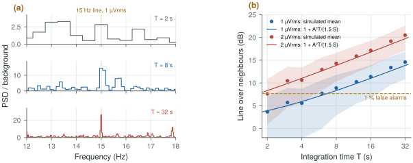
figsrc/ch25_figs.py.The stimulus and the sample clock must agree. A relative error \(\varepsilon\) moves the line by \(\varepsilon f_0\); at half a bin the Hann window loses 1.42 dB, at a whole bin 6 dB. At 15 Hz half a bin is 0.42 % for 8 s and 0.10 % for 32 s: clock the stimulus from the chip’s reference, as for evoked responses in Chapter 33, or search the neighbouring bins.
SSVEP and motor imagery both rely on band power, not on microvolt waveform detail, and both benefit more from more channels and better electrode contact than from more bits.
25.6Features instead of samples
Features pay for themselves in transmission (Chapter 27): the chip makes eight channels of 16-bit words at 500 S/s; a detector needs a few numbers per channel every 2 s.
- Raw: \(8 \times 500 \times 16 = 64\) kb/s.
- Band powers: five bands and the total per channel per 2 s epoch at 16 bits, \(8 \times 6 \times 16/2 = 384\) b/s, 167 times less. (Chapter 27’s 85 times assumes a 256 S/s stream.)
- 8-bit log codes in 0.25 dB steps span 64 dB, from 0.28 µVrms, the input noise in the narrowest band, to a full-scale sine, and round by only 0.07 dB rms against more than 1 dB of scatter: 192 b/s, 333 times less.
- Radio, with Chapter 27’s order-of-magnitude model (5 nJ per bit, 10 µJ per connection event): raw, about 0.4 mW at a 100 ms interval, eight times the 54 µW of the eight channels (Chapter 29); band powers once per epoch, 1.9 µW in bits and 5 µW in events. Five epochs per packet bring that to about 3 µW; a detection flag can still wake the radio at once.
The two estimators also differ in memory. Welch buffers at least one segment: 32–64 kbit for eight channels of 1–2 s at 250 S/s and 16 bits. Fourth-order band-pass filters in 24-bit fixed point (Chapter 23) hold 3.8 kbit of state for five bands on eight channels; the analog servo loop already sets delta’s 0.5 Hz edge.
Keep the full 16-bit, 1.5 µVrms chain for clinical recording, where the raw EEG is read by a person. For on-chip detection, compute band powers, which in this example need only 6–7 bits; that lets the chip send detections and features instead of raw data, which is where the power savings are (Chapter 27). Choose features by testing them against noise: line length looks cheap but responds to noise as strongly as to rhythms. Detect artefacts on chip and flag them; leave ICA to offline analysis. Send band powers as log codes in batches: then the radio’s wake-ups, not the bits, set its power.
On-chip EEG features per channel: band powers (delta to gamma) from a filter bank and squarer over 1–2 s windows, computed on the 500 S/s output decimated to 250 S/s with 8-bit inputs to the feature path, sent as 8-bit log codes (192 b/s for eight channels at 2 s epochs); a threshold or linear detector with per-patient thresholds; artefact flags from amplitude, slope and the DC servo monitor. Raw 16-bit data available on demand.
Reporting window accuracy on data where most windows are negative. With 75 % of windows free of seizures, a detector that never fires is 75 % accurate. Report sensitivity per seizure, detection latency and false detections per hour, and always compare with the trivial detector.
Lab 12 computes band-power features on CHB-MIT, trains a simple classifier, and plots latency and accuracy against word length and sample rate. Start by running figsrc/ch25_figs.py on a CHB-MIT record instead of the synthetic EEG, and replace window accuracy with per-seizure sensitivity and false detections per hour. python figsrc/ch25_figs.py welch ssvep numbers redraws the spectra and the SSVEP study and prints every number of sections 25.4–25.6.
Read with this chapter. The CHB-MIT Scalp EEG Database [32], Verma et al. [25], Buzsáki, Anastassiou and Koch [36] (the origin of the EEG rhythms), Welch [63] (the averaged periodogram), Picton et al. [61] (detecting steady-state responses).
- EEG features are mostly band powers over 1–2 s windows, from Welch spectra or filter banks.
- A Welch bin scatters as \(1/\sqrt{K}\), a band power as \(1/\sqrt{BT}\) (1.4 dB for alpha over 2 s); a filter and squarer uses the whole window and keeps false detections down.
- Artefacts (EOG, EMG) are larger than the EEG; ICA removes them offline, on chip they are flagged.
- In a synthetic study, theta power detects seizure-like discharges at 99 % window accuracy with 6–7 bits; line length fails against noise, though on a real record it does best.
- Inside a band the brain’s background outweighs the 1.5 µVrms floor except in gamma; 8-bit inputs suffice for band powers.
- SSVEP and motor-imagery BCIs rely on band power too; channels and contact quality matter more than bits. A steady-state line gains 3 dB per doubling of time.
- The 16-bit chain is for raw clinical EEG; on-chip detection can run on far fewer bits and send far less data: 192 b/s instead of 64 kb/s.