Chapter 18The SAR ADC
Binary search in silicon: the 12-bit asynchronous SAR is the converter for the multiplexed EMG and spike modes of Open-BioAFE.
- implement the binary search algorithm with a CDAC, a comparator and SAR logic;
- choose between synchronous and asynchronous timing;
- write the SAR logic in Verilog and synthesise or hand-build it;
- add redundancy with non-binary weights and calibrate digitally;
- power-gate and duty-cycle the converter between biosignal samples.
What SAR design reaches 12 bits at the lowest energy per conversion for eight multiplexed channels?
Chapters 15–17 built the parts: a bootstrapped sampler, a 4 pF capacitive DAC of 1 fF units, and a dynamic comparator. This chapter connects them with a few hundred gates of logic, and adds the redundancy and calibration that let the small DAC reach 12 bits.
18.1The binary search algorithm
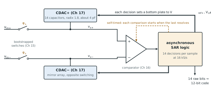
After sampling, the converter knows only that the input lies somewhere in the full range. It tries the midpoint: the MSB capacitor is switched so that the top plate moves by half the reference, and the comparator says whether the input is above or below. The MSB is kept or removed accordingly, and the next bit tries half of what remains. After \(N\) comparisons the DAC’s code is the input to within an LSB. Figure 18.1 shows the blocks that carry out this search in the Open-BioAFE converter.
\(M\) is the number of comparison cycles: \(N\) for a binary array, more with redundancy. For the Open-BioAFE SAR, eight channels at 2 kS/s mean 16 000 conversions per second, 62.5 µs each. Each cycle could take up to 4 µs, a hundred times more than the circuits need, so the SAR converts in a short burst and sleeps for the rest of the period (section 18.5).
18.2Synchronous versus asynchronous timing
A synchronous SAR steps through its cycles on an external clock of at least \(M\) times the conversion rate. Every cycle must be long enough for the slowest one, usually the MSB’s DAC settling and the comparator’s longest, near-metastable decision. Simple, but the clock runs at a rate set by the worst case.
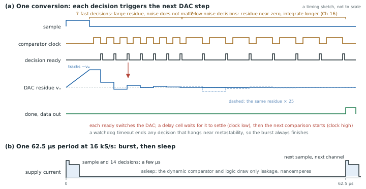
An asynchronous SAR generates its own timing. The comparator signals when it has decided, and that signal triggers the next DAC step and the next comparison. Easy decisions finish quickly, the clock distribution disappears, and only one external pulse per conversion is needed. It needs a timeout, so that a metastable decision (Chapter 16) cannot stall the conversion, and a delay line that guarantees the DAC has settled before each comparison. At biosignal rates either works; asynchronous timing saves the clock’s power and lets the whole burst finish in a few microseconds.
Figure 18.2 shows the burst. After sampling, each decision switches the DAC, a delay cell waits for the residue to settle, and the next comparison starts. The first seven decisions see a large residue and can be fast and noisy; the last seven see a residue near zero and use the comparator’s slower low-noise mode (Chapter 16). Then the converter sleeps until the next sample.
figsrc/ch18_timing_svg.py.18.3SAR logic
The logic is a shift register that walks a “current bit” pointer from the MSB down, and a register that keeps or clears each bit according to the comparator. In Verilog the heart of it is a few lines:
// One SAR step per comparator decision (asynchronous: clk = comparator ready)
always @(posedge clk or posedge start) begin
  if (start) begin                 // new conversion: try the MSB
    ptr  <= 1 << (M-1);
    code <= 1 << (M-1);
  end else if (ptr != 0) begin       // comp = 1: input above the trial level
    code <= (comp ? code : (code & ~ptr)) | (ptr >> 1);  // keep or drop, try next
    ptr  <= ptr >> 1;
  end
end
assign done = (ptr == 0);
code drives the DAC switches directly, through level shifters and drivers sized for the bottom-plate capacitances. The logic can be synthesised with the SG13G2 standard cells and placed by the digital flow (Chapter 30), or built by hand from dynamic logic for the lowest energy. At 16 kS/s, synthesised static CMOS costs about 1.5 pJ per conversion, a fifth of the converter’s energy, which is acceptable.
18.4Redundancy and calibration
Chapter 17 left the DAC with 0.98 fF units whose 1.24 % mismatch puts 0.8 LSB of DNL at mid-scale. Two digital techniques recover the resolution.
Calibration measures the actual weight of each capacitor once, at power-up, by converting known combinations with the converter itself, and stores the weights. Each conversion’s bits are then summed with the measured weights instead of the ideal powers of two.
Redundancy uses more cycles than bits, with weights of radix below two: a 12-bit converter with 14 cycles of radix 1.8 has weights 1820, 1011, 562, … units. Each bit’s weight is now smaller than the sum of all the bits after it, so a wrong early decision, caused by noise, incomplete settling or a too-large MSB, can be corrected by the later bits. That makes calibration always possible (there are no gaps in the transfer curve), and it allows the early decisions to be fast and noisy.
Try the two kinds of search below. Step through a conversion, then switch on the comparator noise: it flips a fast decision only when the residue is already small, and the binary search cannot undo that, because its later steps add up to less than the step just taken. The radix-1.8 search has 25 % to spare after every step, and recovers. Convert 1000 inputs counts the damage for both.
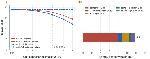
A behavioural Monte Carlo (figsrc/ch18_figs.py) converts a near-full-scale sine with SG13G2-sized units (\(\sigma_u = 1.24\) %) and a comparator with LSB/4 of noise (Figure 18.3a). The median effective resolution is:
- binary, 12 cycles: 11.5 bits uncalibrated, 11.8 bits with calibrated weights;
- radix 1.8, 14 cycles: 11.3 bits uncalibrated, 11.8 bits calibrated.
Uncalibrated, the redundant array is worse, because its non-binary weights do not add up to a uniform code. Calibrated, both reach the noise limit. Redundancy pays for its two extra cycles elsewhere: it guarantees a gap-free curve for every die, not just the median one, and it lets the early decisions use the fast, noisy comparator mode of Chapter 16. Only as many as the redundancy allows, though: with integer weights of 1, 2, 3, 5, 9, 17, 30, 55, … units, the lowest decisions can absorb only 0–4 LSB of error, less than the fast mode’s 0.6 mV (2.5 LSB) of noise. Lab 8 finds a median of 10.0 effective bits with three low-noise decisions, 11.0 with seven and 11.4 with all fourteen (comparator and kT/C noise included); seven low-noise decisions are the design point.
figsrc/ch18_figs.py; the logic and sampler figures are estimates.18.5Power gating and duty cycling
A biosignal SAR spends most of its time doing nothing. With asynchronous timing the 14 cycles finish in a few microseconds, leaving most of the 62.5 µs period idle. Everything with static current should be off during that time: the comparator’s bias (if it has any), the reference buffer’s fast path, the bootstrap charge pumps. Dynamic logic and dynamic comparators draw nothing when not clocked, which is why they suit the job. Leakage is then the floor. In 130 nm thin-oxide logic, a few hundred gates leak only nanoamperes at body temperature, but more at 85 °C (Chapter 15).
The energy per conversion adds up to about 11.7 pJ (Figure 18.3b): comparator 8.0 pJ (seven low-noise decisions at 1.06 pJ and seven fast ones at 0.08 pJ, from the SG13G2 StrongARM of Lab 7), SAR logic 1.5 pJ, CDAC switching 0.84 pJ, average reference charge 0.84 pJ, sampler and timing 0.5 pJ. At 16 kS/s that is 0.19 µW for all eight channels, 23 nW per channel. With 11 effective bits the Walden figure of merit is \(11.7\ \text{pJ}/2^{11} = 5.7\) fJ per step, inside the 10 fJ/step target of Chapter 14.
18.6Case study: a 12-bit SAR in a seizure-detection SoC
The EEG acquisition SoC of Verma et al. [25] is a useful reference design to read alongside this chapter. It multiplexes many EEG channels into a low-voltage SAR converter, chops its front-ends, and computes seizure-detection features on chip. While reading it, look for the choices this chapter discussed: how the sampling capacitor is sized against \(kT/C\) and leakage, how the DAC is switched, how the converter is clocked and duty-cycled, and how much of the total power the converter takes compared with the front-ends and the digital processor. Then compare with the open 12-bit SAR of Moser and Pretl in SKY130 [24], whose schematics, layout and verification are public, and with the 8-bit synchronous SAR of the IHP Analog Academy in SG13G2 [23].
Convert in a fast asynchronous burst and sleep for the rest of the period, so nothing with static current runs between samples. Build the DAC from small units, about 1 fF, and recover the linearity digitally: 14 redundant cycles of radix 1.8 and weights calibrated at power-up give 11 bits or more for every die and allow the early decisions to be fast and noisy, as many as the redundancy can absorb. Expect the comparator to dominate the energy, then the logic. A converter at about 12 pJ per conversion, 0.19 µW for eight channels, is negligible beside the front-ends.
12-bit asynchronous SAR, 14 cycles at radix 1.8 with foreground weight calibration, 16 kS/s shared by eight channels (2 kS/s each; 25 kS/s for one channel in spike mode), ENOB ≥ 11 with seven low-noise comparator decisions, about 11.7 pJ per conversion (5.7 fJ/step), duty-cycled with a burst of a few microseconds per sample.
Calibrating with the converter’s own noise in the loop. A weight measured from a single conversion inherits the comparator’s noise and freezes it into every later conversion. Average each calibration measurement over many conversions (64 or more), and repeat the calibration when the temperature changes by more than a few degrees.
Lab 8 builds the SAR: bootstrapped sample-and-hold, monotonic CDAC, Verilog SAR logic, mixed-signal simulation and adctest.py. Before the transistor-level work, run figsrc/ch18_figs.py with your own unit size and comparator noise to see what ENOB to expect.
Read with this chapter. Verma et al. [25], Moser and Pretl [24], the IHP Analog Academy SAR module [23], Pelgrom [9] (SAR converters).
- A SAR makes \(M \ge N\) comparisons per conversion; at 16 kS/s there is time for a hundred times slower circuits, so the converter runs in bursts and sleeps.
- Asynchronous timing removes the fast clock and adapts each cycle to its decision; it needs a metastability timeout.
- Calibrated weights recover the small DAC (0.98 fF units) to 11.8 bits; a redundant radix-1.8 array with 14 cycles guarantees it for every die and tolerates noisy early decisions.
- The energy is about 11.7 pJ per conversion, dominated by the comparator: 5.7 fJ/step and 0.19 µW for eight channels. The redundancy sets how many decisions may use the fast comparator mode: seven of fourteen.