Chapter 23A DSP Toolkit for Biosignals
Most of what a clinician sees has been filtered, decimated and cleaned after the ADC. The filters must not distort the waveform features they are meant to reveal.
- choose sample rates for each biosignal;
- compare FIR and IIR filters and use zero-phase filtering;
- remove baseline wander and mains interference with adaptive and comb notch filters;
- use wavelets for denoising and feature extraction;
- predict fixed-point effects and choose word lengths;
- estimate the delay, arithmetic and power each filter costs on chip.
Which filters, at what word length, clean each biosignal without distorting it, and how much do they cost on chip?
Part III ends with numbers: 16-bit samples at 500 S/s for ECG and EEG, 12-bit samples at 2 kS/s for EMG. Part IV turns them into information, a heartbeat, a seizure, a gesture, either on the chip or after a radio link. This chapter collects the tools the later chapters share. Tompkins’s book [28] is the classic reference for all of them.
23.1Sample-rate choices
The converters deliver fixed rates (Table 13.1). Each application then keeps only what it needs:
- diagnostic ECG: 500 S/s for 0.05–150 Hz; morphology (ST segments, QRS width) needs the full band and the low corner;
- monitoring ECG: 125–250 S/s for 0.5–40 Hz; heart rate and rhythm survive heavy filtering;
- EEG: 256 S/s for 0.5–100 Hz; seizure features live below 30 Hz;
- EMG: 1–2 kS/s for 10–500 Hz; gesture features are computed over windows of 100–250 ms;
- spikes: 20–30 kS/s for 0.3–7 kHz, reduced to spike times and waveforms before transmission.
Reducing the rate after filtering, decimation, is the cheapest data reduction there is, and it comes before any other processing on chip. The filter in front of it must stop everything that would fold into the kept band; a cascaded integrator–comb (CIC) filter does most of that with additions alone (Chapter 20).
23.2FIR, IIR and zero-phase filtering
FIR filters can have exactly linear phase, so every frequency is delayed by the same time and the waveform’s shape survives, but they need many taps for sharp responses at low frequencies. IIR filters reach the same sharpness with a handful of coefficients, but their phase is nonlinear, and they distort waveforms.
The classic example is the ST segment, the stretch between the QRS complex and the T wave whose level a cardiologist reads for ischaemia. A causal high-pass filter strong enough to remove baseline wander also tilts the ST segment.
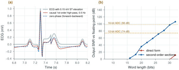
Add a 0.15 mV ST elevation to the synthetic ECG and measure it, relative to the PR baseline, after a first-order high-pass (Figure 23.1a):
- causal, 0.5 Hz: 0.107 mV, 29 % low;
- zero-phase (forward and backward), 0.5 Hz: 0.131 mV, 13 % low;
- causal, 0.05 Hz: 0.146 mV, within 3 %.
The 0.05 Hz corner that the diagnostic ECG standards specify exists for this reason. Monitoring ECG can use 0.5 Hz because it needs only the beats.
figsrc/ch23_figs.py.Zero-phase filtering runs the same IIR filter forwards and then backwards over the record, cancelling its phase. It needs the whole record, or at least a block of it, so it works offline or with a delay, not in a real-time loop.
Linear phase has a price too, paid in time. A symmetric FIR of \(N\) taps delays every frequency by \((N-1)/2\) samples, and \(N\) grows as the narrowest transition band shrinks:
Here \(A\) is the stop-band attenuation in decibels and \(\Delta f\) the narrowest transition band; the tap count is Kaiser’s estimate, as in scipy.signal.kaiserord(). The sample rate cancels: decimation cuts taps and arithmetic, never delay.
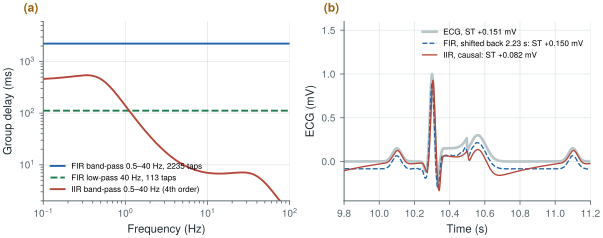
Band-pass the ECG of Worked Example 23.1 to 0.5–40 Hz at 500 S/s, with 40 dB of stop-band attenuation and a 0.5 Hz transition (Figure 23.2):
- Linear-phase FIR: 2,235 taps (Kaiser window) and 2.23 s of delay at every frequency. Shifted back, it reads the ST elevation as 0.150 mV (0.151 mV at its input). At 125 S/s it needs 561 taps and still delays by 2.24 s.
- IIR, a 4th-order Butterworth in two second-order sections: 7 ms of delay for the QRS, but 140 ms at 1 Hz and 461 ms at 0.5 Hz. Run causally, it reads the ST elevation as 0.082 mV, 45 % low.
- Split: for monitoring, let the analog servo set the low corner (Chapter 10) and keep a 40 Hz FIR low-pass with a 10 Hz transition: 113 taps, 112 ms, still linear phase.
Two seconds of delay are harmless in a recording, not in an alarm or a closed loop.
figsrc/ch23_figs.py.23.3Baseline wander and mains interference
Baseline wander, from breathing and electrode motion, sits below about 0.5 Hz. Besides a high-pass filter, two nonlinear methods remove it: fit a spline through the PR segments of successive beats and subtract it, or subtract a median-filtered version of the signal over a window longer than the waves it should ignore. The spline needs the beats to be found first (Chapter 24); the median does not, but it can move the ST segment.
Add respiratory wander, 0.5 mV at 0.25 Hz plus 0.2 mV at 0.08 Hz, to the ECG of Worked Example 23.1, whose ST elevation reads 0.151 mV without it. Remove the wander and read the ST level again:
- causal 0.5 Hz high-pass: 0.107 mV;
- two-stage median, 200 ms then 600 ms (to ignore the QRS, then the P and T waves): 0.026 mV;
- one median over 1.5 s: 0.103 mV;
- cubic spline through the PR segments: 0.151 mV.
At 72 beats/min with 3 % RR variability: 0.116, 0.043, 0.105 and 0.152 mV (0.152 mV without wander). A median follows whatever fills more than half its window: the QRS, ST segment and T wave fill 60 % of a 600 ms window centred on the ST segment, and a longer window works only while the baseline stays flat across it. The spline, anchored at the isoelectric PR segments, never sees the ST segment.
Mains interference at 50 or 60 Hz and its harmonics is what remains after the analog chain’s CMRR and right-leg drive (Chapter 12). A fixed notch drifts off the mains frequency, which varies by a few tenths of a hertz, and rings after artefacts. An adaptive notch [51] instead synthesises a sine at the measured mains frequency, adjusts its amplitude and phase with a least-mean-squares loop to match the interference, and subtracts it, tracking slow changes. A comb filter, a delay of one mains period subtracted from the signal, removes all the harmonics at once, at the price of notches at every multiple of 50 Hz, including some in the EMG band.
The fixed notch is one second-order section with its zeros on the unit circle at the mains frequency and its poles just inside, at radius \(r\):
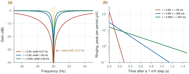
The pole radius sets both the width and the time constant \(\tau\) with which the notch settles and rings: a narrow notch is a slow one. Away from the notch the gain is within 0.1 dB of one for \(r \ge 0.99\).
At 500 S/s the mains sits at \(\omega_0 = 0.2\pi\) (36°), so \(2\cos\omega_0 = 1.618\) (Figure 23.3):
- \(r = 0.95\): 8.1 Hz wide, \(\tau = 40\) ms; 26 dB at 50.2 Hz, but 147 µV of ringing after a 1 mV step artefact and up to 39 µV of error on each 1 mV QRS;
- \(r = 0.99\): 1.6 Hz wide, \(\tau = 0.2\) s; 12 dB at 50.2 Hz, 32 µV of ringing, 8 µV on the QRS; mains that switches on falls to 1 % in \(4.6\tau = 0.92\) s;
- \(r = 0.995\): 0.8 Hz wide, \(\tau = 0.4\) s; only 7 dB at 50.2 Hz, and 16 µV of ringing that lasts twice as long.
A fixed notch is either narrow or tolerant of a ±0.2 Hz drift; an adaptive notch centres itself on the mains, leaving \(r\) to trade width against ringing. With the fixed-point model of Figure 23.1b, the \(r = 0.99\) notch is within 81 dB of floating point at 20 bits and 105 dB at 24; 12 fractional coefficient bits place its centre within 0.008 Hz of 50 Hz (8 bits: 0.13 Hz).
figsrc/ch23_figs.py.The Open-BioAFE mains filter is one section per harmonic (50 and 100 Hz) at \(r = 0.99\), 1.6 Hz wide at 500 S/s, in 24-bit arithmetic, centred on the measured mains frequency; 60 Hz changes only \(2\cos\omega_0\). Make it switchable and keep it out of the raw diagnostic stream. ST-preserving baseline removal belongs to the beat detector of Chapter 24 or to the host.
23.4Wavelets
A wavelet transform splits a signal into octave bands with good time resolution at high frequencies and good frequency resolution at low frequencies, which suits biosignals made of short events on slow backgrounds. Two uses dominate. Denoising: transform, shrink the small coefficients that are mostly noise, and transform back, which removes noise without the blurring of a low-pass filter. Feature extraction: the QRS complex concentrates in the scales around 10–40 Hz, so a QRS detector can work on those coefficients alone. On chip, a lifting implementation of a short wavelet needs only additions and shifts.
23.5Fixed-point effects
On-chip filters run in fixed point, and three effects set the word length.
- Coefficient quantisation moves the poles. A filter whose poles sit very close to the unit circle, such as a high-pass at 0.5 Hz with 500 S/s (poles at 0.994), is extremely sensitive.
- Round-off noise is added at every multiplication and grows with the filter’s internal gain.
- Limit cycles: small oscillations that a recursive filter sustains with zero input because of rounding.
A 4th-order Butterworth high-pass at 0.5 Hz, at 500 S/s, implemented in fixed point (Figure 23.1b):
- in direct form, its expanded polynomial coefficients are so sensitive that it is unstable at every word length up to 30 bits;
- as second-order sections, it reaches 71 dB, the level of a 12-bit converter, at 26 bits, and 97 dB at 30 bits.
Decimating to 125 S/s first, then filtering, moves the poles away from \(z = 1\) by a factor of four and saves several bits. Better still, let the analog DC servo loop (Chapter 10) do the sub-hertz high-pass and keep the digital filters for corners well above 1 Hz.
The notch of Worked Example 23.4 reaches 81 dB at 20 bits; this high-pass needs 28. For a pole pair at \(re^{\pm j\theta}\), an error \(\delta\) in either denominator coefficient moves the pole angle by about
\[\delta\theta \approx \frac{\delta}{2r\sin\theta}.\]The notch’s poles sit at 36° (\(\sin\theta = 0.59\)), the high-pass’s at angles of 0.19 and 0.46 Hz (\(\sin\theta\) = 0.0024 and 0.0058): 100 to 250 times more sensitive, seven to eight bits. Decimating to 125 S/s quadruples \(\theta\), and the high-pass then reaches 76 dB at 24 bits and 91 dB at 26, about three bits better.
23.6What the filters cost on chip
Every filter here costs a fixed number of multiply-accumulates (MACs) per sample: five per second-order section, about \(N/2\) for a symmetric FIR of \(N\) taps, which also stores \(N\) samples, and for a decimating FIR only the outputs kept. Multiply by the sample rate, the channels and an energy per MAC to get power.
Assume 10 pJ per 24-bit MAC with its register traffic, an order-of-magnitude assumption for 130 nm at 1.2 V, not a simulated number. Per channel in ECG mode:
- IIR: 40 Hz low-pass (two sections) plus 50 and 100 Hz notches at 500 S/s, low corner in the analog servo: 10,000 MAC/s, 0.10 µW;
- the FIR band-pass of Worked Example 23.2 at 500 S/s: 559,000 MAC/s, 5.6 µW, and 36 kbit of sample memory;
- the same after decimating to 125 S/s (561 taps): 35,000 MAC/s, 0.35 µW;
- a decimator to 125 S/s (43 taps, 60 dB) plus a 29-tap 40 Hz low-pass: 4,600 MAC/s, 0.05 µW.
Chapter 29 budgets 0.3 µW per channel for decimation and features. The IIR chain uses a third of it; the full-rate FIR needs 19 times as much, 45 µW for eight channels, more than half the 80 µW of the whole analog front-end. Against the 320 µW of streaming raw ECG over a BLE-class radio (Chapter 27), all of them are cheap.
At a few hundred samples per second, register leakage may rival switching; synthesis in the flow of Chapter 30 replaces both estimates with real numbers.
Decimate first, to the lowest rate each application needs. Use zero-phase or linear-phase filtering wherever waveform shape matters, and keep diagnostic high-pass corners at 0.05 Hz. Remove mains interference with an adaptive notch that tracks the mains frequency, not with a fixed one. Implement every recursive filter as second-order sections, and leave sub-hertz corners to the analog servo loop, because at 500 S/s they cost more than 26 bits in fixed point. On chip, run what is causal, short and cheap: decimators, IIR sections, the notch, feature extraction. Send raw samples to the host for sub-hertz linear phase, spline baselines or whole-record processing.
On-chip DSP: decimation to the application rate, second-order-section IIR filters above 1 Hz in 24-bit fixed point, an adaptive 50/60 Hz notch (\(r = 0.99\)), and feature extraction (Chapters 24–26), about 0.1 µW of filtering per channel. Sub-hertz high-pass in the analog servo loop. Diagnostic-quality raw data available at 500 S/s with no on-chip high-pass beyond 0.05 Hz.
Designing an IIR filter in floating point with scipy.signal.butter() and porting its b, a coefficients directly to hardware. For low corner frequencies the direct form is unstable in any practical word length. Always design with output="sos", simulate the fixed-point version, and check stability and limit cycles before committing it to silicon.
In figsrc/ch23_figs.py, decimate the input to 125 S/s before the high-pass and repeat the word-length sweep. Then replace the first-order high-pass of panel (a) with a median-filter baseline removal and measure the ST level again. In fig_notch(), set \(r = 0.98\) and check its width and time constant against the key equation.
Read with this chapter. Tompkins [28]; Widrow et al. [51] for adaptive noise cancelling and the adaptive notch; Haykin [52] for the least-mean-squares algorithm.
- Decimate to the application’s rate first: 500 S/s for diagnostic ECG, 125–250 S/s for monitoring, 256 S/s for EEG.
- A causal 0.5 Hz high-pass reads a 0.15 mV ST elevation as 0.107 mV and a two-stage median baseline filter as 0.026 mV; zero-phase filtering, a 0.05 Hz corner or a spline through the PR segments preserves it.
- A linear-phase FIR delays by \((N-1)/2\) samples, 2.2 s for a 0.5 Hz transition at any rate; a causal IIR band-pass reads the ST elevation 45 % low.
- A 50 Hz notch with \(r = 0.99\) at 500 S/s is 1.6 Hz wide and settles with \(\tau = 0.2\) s. Adaptive notches track the mains frequency; comb filters remove all harmonics at the cost of extra notches.
- Wavelets denoise without blurring and isolate the QRS scales.
- Narrow recursive filters need second-order sections and long words: 26 bits for 12-bit quality at 0.5 Hz and 500 S/s, about eight more than a 50 Hz notch.
- On chip, IIR filtering costs about 0.1 µW per channel at an assumed 10 pJ per MAC; a full-rate linear-phase band-pass would cost 5.6 µW.