Chapter 14Specifications, Figures of Merit and Architecture Choice
A converter is described by a dozen numbers, but for a biosignal chip two of them, resolution and energy per conversion, decide the architecture.
- define SNR, SNDR, SFDR, THD, ENOB, DNL, INL, offset and gain error and measure each;
- compute the Walden and Schreier figures of merit and know when each applies;
- place biomedical converters on the Murmann ADC survey;
- explain why thermal-noise-limited power grows \(\times 4\) per bit and \(CV^2\)-limited power \(\times 2\);
- choose between SAR, ΔΣ, incremental, VCO-based and event-driven converters for a given biosignal.
Which converter architecture fits each Open-BioAFE mode, and what energy per conversion should you expect?
Chapter 13 found the rates and resolutions an ideal converter would need: 16 bits at a few hundred samples per second for ECG and EEG, 12 bits at 2 kS/s for EMG (Table 13.1). Real converters fall short of the ideal in ways that have names and standard measurements. This chapter defines them, then asks what the converter will cost in energy, because that, more than speed, is what limits a converter on a body-worn chip.
14.1Dynamic and static specifications
Dynamic specifications come from the spectrum of a sine wave converted at full speed. Take an FFT of the output codes and sort its bins into four groups: the bin that holds the input tone, the bins that hold its harmonics, the DC bin (ignored) and everything else, which is noise.
SNDR is the single number that matters most, because it counts every error. Its equivalent in ideal bits is the ENOB of Chapter 13, \((\mathrm{SNDR} - 1.76)/6.02\). SFDR is the distance from the signal to the tallest unwanted line, noise or harmonic, and it matters when a small signal must be seen next to a large one at another frequency, as an EEG rhythm next to a mains harmonic.
The FFT only sorts the bins cleanly if the tone completes a whole number of cycles in the record. Choose the input frequency as
\[f_\mathrm{in} = \frac{M}{N_\mathrm{FFT}}\,f_\mathrm{s}, \qquad M \text{ odd and coprime with } N_\mathrm{FFT},\]and all the signal power falls into bin \(M\), the codes visit as many different levels as possible, and no window is needed. This is coherent sampling, done by biosig.coherent_tone(). When it is not possible, for example when you record a real ECG, a window such as the Hann window spreads the tone over a few bins and the metrics are computed from those bins; Chapter 22 treats both cases in full.
Static specifications describe the transfer curve itself, measured slowly. An ideal converter changes code every LSB. A real one has code widths \(W_k\) that differ:
- the differential nonlinearity of code \(k\) is \(\mathrm{DNL}_k = W_k/\Delta - 1\); a DNL of −1 LSB means the code never appears, a missing code;
- the integral nonlinearity is the running sum of the DNL, the distance of each transition from a straight line through the end points (or through a best fit);
- offset and gain error shift and tilt the whole curve.
The easiest way to measure DNL is a code-density histogram: drive the converter with a slow, uniform ramp and count how often each code appears. A wide code catches more samples than a narrow one, so the counts, divided by their mean, are \(1 + \mathrm{DNL}_k\). biosig.dnl_inl() does this; a sine input works too, with a correction for its arcsine distribution (Chapter 22).
Offset and gain error matter less in a biomedical channel than in an instrument. The converter’s offset adds to the electrode offset that the high-pass and the DC servo loop already remove (Chapter 10), and a gain error of a few percent is calibrated with one digital multiplication per channel. DNL and INL cannot be calibrated so easily, because they differ code by code.
A SAR converter (Chapter 18) compares its input with a binary-weighted capacitor DAC. Build the 12-bit DAC from 4096 unit capacitors, the MSB from 2048 of them, and let each unit scatter by \(\sigma_u = 1\,\%\). The MSB weight then scatters by \(\sigma_u\sqrt{2048} = 0.45\) LSB. At mid-scale, where the code steps from 2047 to 2048, the converter compares the MSB against all the other bits together, so the error of that one step is the difference of two sums of about 2048 units:
\[\sigma_\mathrm{DNL,mid} \approx \sigma_u\sqrt{2^N} = 0.01 \times 64 = 0.64\ \text{LSB}.\]biosig.sar_convert() with the weights from biosig.cdac_weights(12, 0.01, seed=2) gives DNL from −0.42 to +1.45 LSB, INL within ±0.85 LSB, and an SNDR of 69.5 dB (11.3 effective bits) with an SFDR of 76.2 dB, against 74.0 dB for the ideal converter (Figure 14.1).
For the mid-scale step to stay within ±0.5 LSB at three standard deviations, \(3\sigma_u\sqrt{2^N} < 0.5\), or \(\sigma_u < 0.26\,\%\). At \(\sigma_u = 0.2\,\%\) the same simulation keeps 11.95 effective bits. Chapter 17 turns this requirement into a unit capacitor size with the SG13G2 matching data.
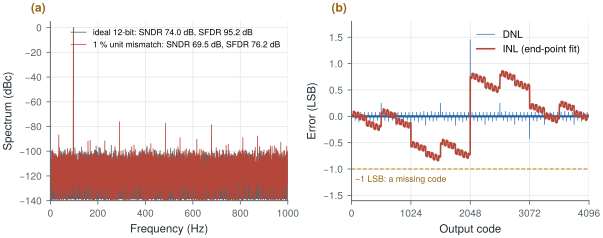
biosig.sar_convert() and biosig.dnl_inl().14.2Figures of merit
Two converters with different resolutions, rates and powers are compared with a figure of merit, a single number that normalises power by what the converter delivers. Two are in common use, and they make different assumptions about how power grows with resolution.
with \(\mathrm{BW} = f_\mathrm{s}/2\) for a Nyquist converter and the signal bandwidth for an oversampled one.
The Walden FoM is the energy per conversion divided by the number of effective levels, in joules per conversion step; lower is better. It assumes that one more bit doubles the energy, which is how a converter behaves when switching energy and logic dominate. The Schreier FoM is in decibels; higher is better. Because SNDR in decibels enters with weight one, it assumes that one more bit (6 dB) costs four times the power, which is how a converter behaves when thermal noise dominates (section 14.3).
SAR, EMG mode. Say the converter reaches 11 effective bits at 2 kS/s with a Walden FoM of 10 fJ per step, good but well short of the best published SARs. Each conversion costs
\[E = 10\ \text{fJ} \times 2^{11} = 20\ \text{pJ}, \qquad P = 20\ \text{pJ} \times 2\ \text{kS/s} = 41\ \text{nW}.\]Eight channels need 0.33 µW, a few percent of one channel’s 10 µW front-end budget.
Incremental ΔΣ, ECG/EEG mode. It needs 98 dB in a 150 Hz band. With a Schreier FoM of 175 dB,
\[P = \mathrm{BW}\cdot 10^{(\mathrm{SNDR} - \mathrm{FoM_S})/10} = 150\ \text{Hz} \times 10^{(98 - 175)/10} = 3.0\ \text{µW}\]per channel, 30 % of the front-end budget. A 180 dB design would need 0.95 µW. And if the DC servo loop lets the converter get by with 90 dB instead of 98 dB, the 175 dB design needs only 0.47 µW: every 10 dB of dynamic range costs a factor of ten in power.
Murmann’s ADC survey [22] collects the published converters since 1997, and plotting their energy per Nyquist sample, \(P/(2\,\mathrm{BW})\), against SNDR shows where the state of the art lies. Figure 14.2b draws the same axes with lines of constant FoM instead of the data points. The best converters in the survey reach a Walden FoM below 1 fJ per step at low and medium resolution and a Schreier FoM above 180 dB at high resolution, and the edge of the cloud bends from the Walden slope to the Schreier slope at around 75 dB. That is why both FoMs survive: the 10 fJ/step and 175 dB lines cross at 74 dB, right at 12 bits. Use the Walden FoM for the SAR and the Schreier FoM for the ΔΣ converter.
14.3Power per bit
The four-times-per-bit rule comes from \(kT/C\) noise. Sampling a voltage on a capacitor \(C\) freezes the thermal noise of the switch with it, a noise power of \(kT/C\) whatever the switch resistance (Chapter 6, Chapter 15). For this noise not to exceed the quantisation noise \(\Delta^2/12\) of an \(N\)-bit converter with range \(V_\mathrm{FS}\):
Each extra bit quadruples the capacitor, and charging it from the supply every sample, \(E \approx CV_\mathrm{DD}^2\), quadruples the energy. The second bound follows from the first: a full-swing sine of power \(V_\mathrm{FS}^2/8\) over a noise of \(kT/C\) needs \(C = 8kT\cdot\mathrm{SNR}/V_\mathrm{FS}^2\), and with \(V_\mathrm{FS} \approx V_\mathrm{DD}\) the charging energy is \(8kT\cdot\mathrm{SNR}\). On the axes of Figure 14.2b it is the solid line, and it corresponds to a Schreier FoM of about 192 dB, which no converter reaches.
With \(V_\mathrm{FS} = 1.2\) V peak to peak and \(kT = 4.14 \times 10^{-21}\) J at 300 K:
- 12 bits at the Nyquist rate: \(\Delta = 293\) µV and \(C \ge 0.58\) pF; the thermal energy bound at 74 dB is 0.83 pJ per sample.
- 16 bits at the Nyquist rate: \(C \ge 150\) pF, a capacitor that would fill a large part of the die for each channel; the bound at 98 dB is 0.21 nJ per sample.
- 16 bits at an OSR of 128: the noise is spread over 128 times the band and \(C \ge 1.2\) pF.
Oversampling is what makes 16 bits affordable: the same capacitor budget that gives a 12-bit Nyquist converter gives a 16-bit oversampled one. It also explains why the 12-bit SAR is not limited by \(kT/C\) at all. Its 0.58 pF total would make each unit capacitor 0.14 fF, far too small to match to 0.26 % (Worked Example 14.1). Matching, not noise, sets the size of its DAC, and with a larger DAC than noise requires, the energy is set by switching that DAC and running the comparator and logic, roughly doubling per bit.
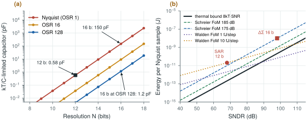
biosig.ktc_cap() and biosig.e_thermal_min().14.4Architecture choice for biosignals
Table 14.1 summarises the options. Each row is a different answer to the same trade-off between energy per conversion, resolution, the analog filtering it needs and how much of it is digital. Figure 14.3 places them on a map of resolution against sample rate.
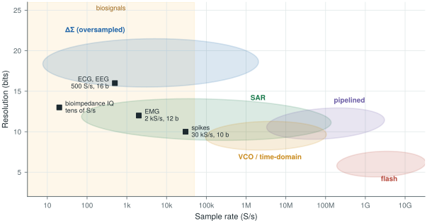
figsrc/ch14_figs.py.Table 14.1. Converter architectures for biosignals. The two converters built in this tutorial are the SAR and the incremental ΔΣ; the others appear in Chapter 21 or only for contrast.
| Architecture | Typical bio use | Strength | Weakness |
|---|---|---|---|
| SAR | Multiplexed ExG, neural spikes, 8–12 b | Lowest energy per conversion, mostly digital, scales with technology | Needs an anti-alias filter and S/H; \(kT/C\) and DAC matching limit the bits |
| ΔΣ (DT or CT) | ECG/EEG at 14–20 b | Relaxed anti-alias filter, high resolution, mismatch-tolerant with a 1-bit DAC | Decimation-filter power; continuous operation; idle tones |
| Incremental ΔΣ | Multiplexed high-resolution channels | ΔΣ accuracy with a reset per sample, multiplexer-friendly | Lower SQNR per OSR than a free-running ΔΣ |
| VCO / time-domain | Direct digitisation, tiny area | Mostly digital, inherent first-order shaping | VCO nonlinearity, supply sensitivity |
| Level-crossing / event-driven | Sparse signals (spikes, ECG) | Data and power scale with activity | Non-uniform samples, harder DSP |
| Pipeline / flash | Not used for ExG | Speed | Power far beyond biosignal needs; shown only for contrast |
The SAR for EMG and spikes. At 12 bits and a few kilosamples per second the SAR sits in the Walden regime, where its mostly digital operation and tiny energy per conversion are unmatched. Its weaknesses are the ones found above: DAC matching limits it near 12 bits, and as a Nyquist-rate converter it needs the anti-alias filter of Chapter 11. Chapters 15–18 build it.
The incremental ΔΣ for ECG and EEG. At 16 bits the converter is in the Schreier regime, and oversampling is the way to pay for the resolution: the sampling capacitor shrinks by the OSR, the anti-alias filter shrinks to a pole or two (Chapter 13), and a 1-bit feedback DAC is linear by construction, so 16 bits need no 16-bit matching. The incremental variant resets its integrators before each conversion. Each output then depends only on its own window of input, as with a Nyquist converter, so it can be multiplexed between channels, carries no idle-tone memory from one sample to the next, and needs a simpler decimation filter. The price is a lower SQNR for a given OSR than a free-running modulator; Chapter 19 gives the theory and Chapter 20 the circuits.
The alternatives. VCO-based converters turn the input into a frequency and count it, so they are almost entirely digital and shape their quantisation noise to first order for free, but the VCO’s nonlinearity and supply sensitivity limit their accuracy. Level-crossing converters sample only when the signal moves by a threshold, so a quiet ECG between beats costs almost nothing. Both are treated in Chapter 21.
The 12-bit SAR costs a few tens of nanowatts per channel and hardly enters the power budget; design it for matching and simplicity. The 16-bit ΔΣ converter costs microwatts, a large fraction of the 10 µW channel budget, and its power scales by ten for every 10 dB of dynamic range. Each decibel of electrode offset or artefact headroom the front-end removes before the converter therefore saves real power. That makes the DC servo loop of Chapter 10 a converter-power decision as much as a front-end one.
SAR (EMG, spikes): 12 bits, ENOB ≥ 11, Walden FoM ≤ 10 fJ per step, so about 40 nW per channel at 2 kS/s. Incremental ΔΣ (ECG, EEG): 16 bits, 150 Hz band, Schreier FoM ≥ 175 dB (goal 180 dB), so 1–3 µW per channel. To be confirmed by the budgets of Chapter 29.
A figure of merit is only comparable within the regime it was made for. The Walden FoM rewards high resolution unfairly: on Figure 14.2b the 1 fJ/step line drops below the thermal bound above about 88 dB, so a “1 fJ/step 16-bit converter” is physically impossible. Also check what the quoted power includes. Oversampled converters often leave out the decimation filter and the reference buffers, and Nyquist converters the input driver, and any of these can cost more than the converter core.
Lab 6 computes SNDR, SFDR and ENOB and histogram DNL/INL with injected capacitor mismatch. Reproduce Worked Example 14.1 with biosig.cdac_weights() and biosig.sar_convert(), then sweep \(\sigma_u\) and find where the first missing code appears.
Read with this chapter. Murmann [22] for the survey data and its plots, Pelgrom [9] for specifications, matching and the energy limits, Schreier, Temes and Pavan [10] for the Schreier FoM and incremental converters.
- SNDR (and the ENOB derived from it) counts every error; SFDR measures the tallest spur; DNL and INL describe the transfer curve code by code.
- Coherent sampling puts the whole tone in one FFT bin; a ramp histogram gives DNL directly.
- In a 12-bit binary capacitor DAC the mid-scale DNL scatters by about \(\sigma_u\sqrt{2^N}\); keeping it within ±0.5 LSB needs unit capacitors matched to 0.26 %.
- Walden FoM assumes ×2 energy per bit (switching-limited, low resolution); Schreier FoM assumes ×4 (thermal-noise-limited, high resolution). They cross near 12 bits.
- \(kT/C\) needs 0.58 pF for 12 bits but 150 pF for 16 bits at the Nyquist rate; oversampling by 128 brings 16 bits back to 1.2 pF.
- Expect about 40 nW per channel for the 12-bit SAR and 1–3 µW for the 16-bit ΔΣ; the ΔΣ is the converter that matters for power.