Chapter 21Biomedical Converter Innovations
In recent designs the boundary between the amplifier and the converter is dissolving.
- explain direct digitisation with ΔΣ front-ends that take the electrode as input;
- design for the large input range that motion artefacts require;
- describe VCO- and time-based ADCs;
- compare level-crossing and event-driven sampling with uniform sampling;
- assess compressive sensing for biosignals.
When does it pay to merge the amplifier and the ADC, and when to sample only on events?
Open-BioAFE follows the classic partition: a chopped LNA, a PGA and filter, then a SAR or an incremental ΔΣ converter. That partition is conservative on purpose, because every block can be designed, simulated and measured on its own. Recent research chips blur it in four ways. This chapter explains each, with the budgets of the earlier chapters in hand.
21.1Direct digitisation
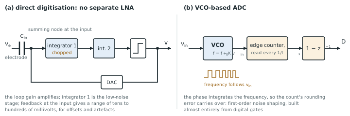
A direct-digitisation front-end has no separate LNA. A ΔΣ modulator takes the electrode voltage as its input, through input capacitors or a transconductor, and its loop gain does the amplifying. The first integrator acts as the low-noise stage, chopped to remove its flicker noise, and the DAC feedback sits at the input (Figure 21.1a).
The motivation is dynamic range. A conventional chain applies a gain of 100 or more before the converter, so a 30 mV motion artefact or a 300 mV electrode offset saturates it, and the channel loses data until the high-pass recovers (Chapter 10). A direct-digitising loop has no gain before the quantiser to saturate. Its input range is set by the DAC and can be hundreds of millivolts, while its noise is set by the first integrator, so it can tolerate the artefact and still resolve the microvolt EEG under it. Chapter 2 found that a DC-coupled channel needs about 103 dB, almost 17 bits; direct digitisation is how recent designs reach that at microwatts.
The costs: the first integrator must meet the front-end’s noise specification and the converter’s linearity at full input range; the input impedance is that of the loop’s input capacitors or transconductor, often switched and low (Chapter 9); and the converter can no longer be designed and tested separately.
21.2VCO- and time-domain ADCs
A voltage-controlled oscillator turns its input voltage into a frequency. Counting its cycles in each sampling period integrates that frequency, and the count’s quantisation error is carried over to the next period, so a VCO-based ADC is a first-order noise-shaping quantiser built almost entirely from digital gates (Figure 21.1b). It needs no precise capacitors, scales with technology, and uses very little area.
Its limit is the VCO’s tuning curve: frequency is not a linear function of voltage, so an open-loop VCO-ADC distorts beyond about 40–60 dB. Putting the VCO inside a ΔΣ loop, where the loop gain suppresses its nonlinearity, or using it only as the quantiser of a conventional loop, recovers the linearity. Supply sensitivity is the other weakness: a ring oscillator’s frequency follows its supply, so the supply must be clean or the measurement made differential with two matched oscillators.
21.3Level-crossing and event-driven sampling
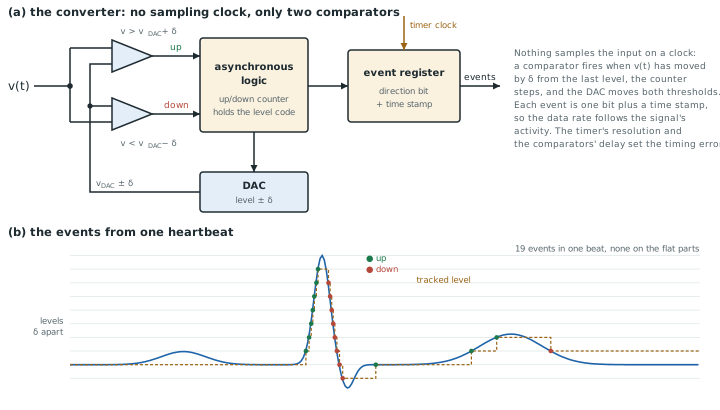
A uniform sampler takes 500 samples per second of an ECG whether the heart is beating or the signal is flat between beats. A level-crossing ADC samples only when the signal has moved by a threshold \(\delta\) since the last sample. It records the time of the crossing rather than the value. Its data rate, and much of its power, follows the signal’s activity.
Figure 21.2 shows how. Two continuous-time comparators watch the input against the DAC level plus and minus \(\delta\). When one fires, asynchronous logic steps an up/down counter, the DAC moves both thresholds by \(\delta\), and an event register stores the direction with a time stamp from a free-running timer. No clock samples the input, so the comparators’ delay and the timer’s resolution set the timing error, and a feature smaller than \(\delta\), like the P wave in the figure, is never seen at all.
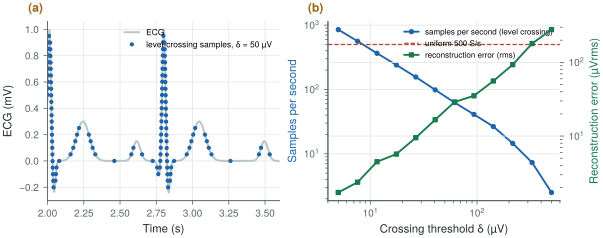
figsrc/ch21_lc_arch_svg.py.figsrc/ch21_figs.py applies an ideal level-crossing sampler to the synthetic 1 mV ECG of biosig.ecg() and reconstructs it by linear interpolation (Figure 21.3):
- \(\delta = 7.6\) µV: 562 samples per second and 2.4 µVrms of error, about the same rate as uniform sampling;
- \(\delta = 27\) µV: 156 samples per second, three times fewer than 500 S/s, with 9.5 µVrms of error, 1 % of the R wave;
- \(\delta = 62\) µV: 62 samples per second and 29 µVrms of error.
Most of the samples fall on the QRS complex, where the signal changes quickly; the flat segments cost almost nothing.
The saving depends entirely on the signal. A sparse ECG or a spike train with long quiet periods benefits; an EEG, which is busy all the time, does not. The samples are non-uniform in time, so the digital processing that follows must either work with irregular samples or resample, and the threshold sets a resolution floor that, at useful compression, is far above the 1.5 µVrms noise target. Level crossing suits feature extraction (heart rate, spike detection) more than diagnostic recording.
figsrc/ch21_figs.py with biosig.ecg().21.4Compressive sensing
Compressive sensing goes further. If a signal is sparse in some basis, such as wavelets for ECG, it can be recovered from far fewer random linear combinations of its samples than its Nyquist rate suggests. The chip computes the random projections, cheaply, with additions and sign flips, and transmits only them; the receiver solves an optimisation problem to reconstruct the signal.
The saving is in the radio, which in a wireless biosignal system often costs more energy per bit than the sensing (Chapter 27). The cost is reconstruction: it is computationally heavy, happens off chip, and degrades gracefully but noticeably as the compression rises. Compression ratios of two to four are realistic for ECG at clinically acceptable error; EEG compresses less. For a chip that does its own feature extraction (Part IV), sending features instead of compressed raw data usually saves more.
21.5The dissolving AFE/ADC boundary
The surveys of converter performance [22] and the biomedical sessions of the major circuit conferences show the same trend year after year: the LNA, the filter and the converter merge into one loop, the converter’s input range grows to swallow artefacts, and more of the work moves to digital logic. When you read such a design, check it with the budgets of this tutorial:
- noise: the input-referred noise over the stated band, and the NEF of the whole channel, not of the first stage (Chapter 6);
- input impedance, measured with the chopper or the switched input running (Chapter 10);
- CMRR with an imbalanced source, not only the amplifier’s own (Chapter 7);
- range: the largest artefact or offset tolerated without losing data;
- energy: what the power figure includes, such as references, clocks, decimation and bias (Chapter 14).
Merge the amplifier and the converter when the input range matters more than modularity: direct digitisation tolerates large artefacts and electrode offsets without saturating, at the price of a first stage that must be both quiet and linear. Sample on events when the signal is sparse and the application needs features rather than morphology: three times fewer ECG samples for 1 % error. Keep the classic partition, as Open-BioAFE does, when each block must be designed, verified and characterised on its own, which is the right choice for a first open-source chip.
Open-BioAFE keeps the classic partition (chopped LNA, PGA, SAR or incremental ΔΣ), with the DC servo loop’s output digitised as an electrode-offset monitor to keep the information a direct-digitising design would capture (Chapter 10). Level-crossing and compressive modes are left for a later revision.
Comparing an event-driven converter with a uniform one by samples per second alone. Each level-crossing sample carries a time stamp as well as a value, and its accuracy depends on the timing resolution; the reconstruction error, not the sample count, is the fair measure. Compare both at the same error, as in Figure 21.3b.
Run figsrc/ch21_figs.py on an EEG from biosig.eeg() instead of the ECG, and compare the samples per second at the same reconstruction error. Then add 5 µVrms of noise to the ECG before sampling and see what happens to the level-crossing rate at small thresholds.
Read with this chapter. Murmann [22] for the survey, Yazicioglu, Van Hoof and Puers [8] for biopotential readout architectures, Schreier, Temes and Pavan [10] for VCO-based quantisers in ΔΣ loops.
- Direct digitisation closes a ΔΣ loop around the electrode: no gain to saturate, large artefact range, but a first stage that must be quiet and linear.
- VCO-based ADCs are digital first-order shaping quantisers; their nonlinearity needs a loop around them.
- Level-crossing sampling of an ECG gives about three times fewer samples than 500 S/s at 1 % error; it suits sparse signals and feature extraction.
- Compressive sensing saves radio energy at the price of off-chip reconstruction; sending features often saves more.
- Check new designs with the same noise, impedance, CMRR, range and energy budgets as a conventional chain.