Chapter 28Bioimpedance Sensing and IQ Demodulation
Inject a small AC current, measure the voltage, and recover the complex impedance of tissue or of the electrode interface.
- model tissue and electrodes with the Cole model and its dispersion;
- explain why a tetrapolar (four-electrode) measurement removes electrode impedance;
- design excitation sources: sine DAC with V-to-I converter, Howland and OTA-based current sources, square and pseudo-sine waves, multi-sine and chirp;
- implement IQ (quadrature) demodulation in the analog and digital domains and predict its errors;
- run ECG and impedance on the same electrodes by frequency separation;
- respect the frequency-dependent patient-current limits.
What excitation frequency, current and demodulator give the required \(\Delta Z\) resolution within the safety limits?
Everything so far has listened to the body. Bioimpedance sensing asks the body a question instead: it injects a known AC current and measures the voltage it produces. The ratio is a complex impedance that changes with breathing, with blood volume, with body composition, and with the state of the electrode contact. That last use, tracking every electrode’s impedance while it records, is the optional impedance-aware channel of Open-BioAFE.
28.1Applications
- Impedance pneumography: breathing changes the thorax’s impedance by of the order of an ohm on a baseline of tens of ohms, measured through the ECG electrodes themselves;
- impedance cardiography: each heartbeat changes it by about a tenth of that, from which stroke volume is estimated;
- body composition (bioimpedance analysis and spectroscopy): the frequency dependence separates intracellular and extracellular water;
- electrical impedance tomography: many electrodes around a body section, reconstructed into an image of conductivity;
- electrodermal activity: skin conductance, which follows sweat-gland activity and arousal;
- electrode-contact quality: the electrode impedance itself, the generalisation of the lead-off detection of Chapter 12;
- cell and tissue impedance spectroscopy in the laboratory.
28.2Tissue and electrode models
Tissue is a mix of conducting fluids and cell membranes that behave as capacitors. At low frequencies current flows around the cells, through the extracellular fluid only; at high frequencies it also passes through them. The Cole model describes the transition:
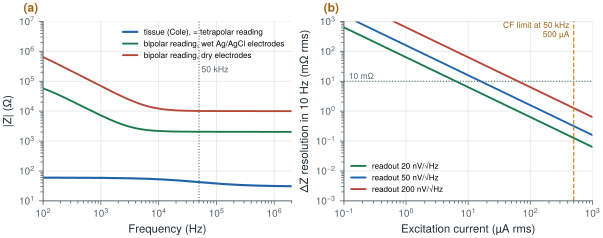
\(R_0\) is the low-frequency (extracellular) resistance, \(R_\infty\) the high-frequency one, \(f_\mathrm{c}\) the characteristic frequency and \(\alpha\) (0.5–1) the spread of cell sizes and shapes. The example of Figure 28.1 uses \(R_0 = 60\) Ω, \(R_\infty = 30\) Ω, \(f_\mathrm{c} = 30\) kHz and \(\alpha = 0.7\): 42 Ω at −12° at 50 kHz.
The electrodes are in series with the tissue, and they are far larger. In a bipolar measurement, where the same two electrodes inject the current and sense the voltage, the reading is \(Z_\mathrm{tissue} + 2Z_\mathrm{e}\): with the wet electrode model of Chapter 3 about 2 kΩ at 50 kHz around 42 Ω of tissue, and about 10 kΩ with dry electrodes. A tetrapolar measurement injects the current through one pair and senses the voltage with a second pair. The sensing pair carries almost no current, so its electrode impedance drops no voltage, and the reading is the tissue alone (Figure 28.1a).
The dynamic range follows: a \(\Delta Z\) of a tenth of an ohm (cardiac) on 42 Ω of tissue, which may itself sit on kilohms of electrode impedance, is a change of a few parts in ten thousand. A readout that subtracts the baseline before amplifying it, like the servo loop of Chapter 10, is what makes it measurable.
The demo below draws the Cole model and the point a 10 µA readout measures. It starts at this section’s example (R0 = 60 Ω, R∞ = 30 Ω, fc = 30 kHz, α = 0.7: 42 Ω at −12° at 50 kHz); switch to a bipolar measurement and see what the electrodes do to it.
28.3Excitation
The excitation should be a current, so that the voltage measured is the impedance times a known value. The options:
- a sine DAC with a voltage-to-current converter: clean, but a DAC and a linear transconductor at tens of kilohertz cost area and power;
- a Howland current source: an op-amp with matched resistors, with an output impedance set by the resistor matching;
- an OTA-based current source on chip, whose output impedance and common-mode control decide how much of the current reaches the body rather than the parasitics;
- square-wave or pseudo-sine excitation from switched current sources: almost free in a CMOS chip, but rich in odd harmonics (section 28.4);
- multi-sine or chirp excitation for spectroscopy, measuring many frequencies at once.
The current must respect the patient-current limits of Chapter 4, which rise with frequency above 1 kHz: for a type CF applied part in normal condition, 10 µA at DC and 1 kHz, and 500 µA at 50 kHz. The excitation must also be balanced, so that its common mode does not appear at the ECG inputs.
28.4IQ demodulation
The measured voltage is a sine at the excitation frequency whose amplitude and phase carry the impedance. IQ demodulation recovers both: multiply the signal by an in-phase and a quadrature reference at the same frequency, and low-pass filter each product. The two DC outputs are the real and imaginary parts of \(Z\), times the current:
This is synchronous detection, the principle of the lock-in amplifier: anything not at the reference frequency, ECG, noise and interference, averages out in the low-pass filter, whose bandwidth sets the noise. The resolution follows directly:
With a readout noise of 50 nV/√Hz at the excitation frequency and a 10 Hz output bandwidth (respiration and heartbeat), the input noise is \(50\ \text{nV} \times \sqrt{10} = 0.16\) µVrms. Dividing by the current (Figure 28.1b):
- 10 µA gives 16 mΩ rms, enough for respiration (of the order of an ohm) but marginal for the cardiac signal (of the order of 0.1 Ω);
- 50 µA gives 3.2 mΩ, a tenth of the limit at 50 kHz, and enough for both;
- 500 µA, the CF limit at 50 kHz, would give 0.3 mΩ.
At 50 µA a 1 Ω change is a 50 µV signal, which a front-end designed for microvolts measures easily.
figsrc/ch28_figs.py.The demodulator can be built three ways, each with its own error:
- analog multipliers: accurate, but linear multipliers at tens of kilohertz cost power;
- square-wave (chopper-style) demodulators: switches that multiply by ±1, essentially free and the natural partner of the choppers of Chapter 9. A square wave contains odd harmonics with weights 1/3, 1/5, …, so it also demodulates any signal at three, five, … times the excitation frequency. With a square-wave excitation as well, the tissue’s response at those harmonics, where its impedance differs, adds an error. A pseudo-sine excitation without third and fifth harmonics, or a sine excitation, removes most of it;
- digital IQ after the ADC: exact multiplication and filtering in logic, but the ADC must sample the excitation frequency and handle the full baseline.
All three suffer from reference phase errors (a phase offset rotates \(I\) into \(Q\), so magnitude is robust but phase is not) and I/Q gain mismatch. Both are calibrated with a known on-chip resistor.
28.5Readout architecture
The readout is an instrumentation amplifier at the excitation frequency, followed by the demodulators and low-pass filters, with a baseline-cancellation loop that subtracts the large static impedance so that the small changes use the converter’s range. The IQ outputs are slow, a few hertz to tens of hertz, so the SAR converter of Chapter 18 digitises them at a fraction of its capacity (Figure 28.2).
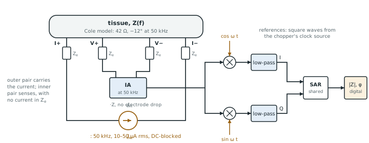
ECG and impedance on the same electrodes work by frequency separation: the ECG lives below 150 Hz, the excitation at tens of kilohertz. The ECG front-end’s low-pass and decimation filters reject the excitation; the impedance demodulator rejects the ECG. The chopper and the excitation must not share a frequency, or harmonics, with each other. Multi-frequency and multi-channel systems, such as EIT, multiplex the excitation and readout across electrode pairs.
For Open-BioAFE’s impedance-aware mode, the same idea runs on every recording electrode at once: one small out-of-band excitation shared by all channels, IQ demodulation timed with the chopper clock, and duty cycling while the contacts are stable, so that each sample carries its own contact-quality figure (Chapter 29). Pallàs-Areny and Webster’s treatment of sensors and signal conditioning [33] and Webster’s chapter on bioimpedance [7] cover the classical background.
Measure tissue with four electrodes, or the electrodes will dominate the reading by fifty to more than two hundred times. Excite at tens of kilohertz, where the patient-current limit is hundreds of microamperes, and pick the current from the resolution you need: 50 µA and a 50 nV/√Hz readout resolve 3 mΩ in 10 Hz. Demodulate synchronously, with square-wave switches if you use a sine-like excitation, and calibrate phase and gain with an on-chip resistor. Cancel the baseline before amplifying the changes.
Optional impedance channel: balanced pseudo-sine current excitation at about 50 kHz, 10–50 µA (well inside the 500 µA CF limit), tetrapolar or electrode-tracking configuration, square-wave IQ demodulators synchronised with the chopper clock, baseline cancellation, IQ outputs digitised by the SAR; ΔZ resolution about 3 mΩ rms in 10 Hz at 50 µA; calibration against an on-chip resistor.
Checking the excitation current against the DC patient-current limit, or only against the limit at the fundamental. A square-wave excitation has odd harmonics, each with its own limit, and a fault can leave a DC component on the electrodes. Check the whole spectrum of the excitation, in normal and single-fault conditions, and block DC with series capacitors.
Lab 15 builds the impedance readout: a Cole tissue model, a tetrapolar measurement and digital IQ in Python, then an SG13G2 current source and a square-wave IQ demodulator. Start from figsrc/ch28_figs.py: add a respiration \(\Delta Z\) of 0.5 Ω at 0.25 Hz to the tissue, demodulate it digitally, and compare analog square-wave demodulation with digital IQ.
Read with this chapter. Pallàs-Areny and Webster [33], Webster [7] (bioimpedance), and the patient-current limits of IEC 60601-1 [41].
- The Cole model describes tissue’s transition from extracellular to total conduction; the example tissue is 42 Ω at −12° at 50 kHz.
- A bipolar reading adds two electrode impedances (about 2 kΩ wet, 10 kΩ dry at 50 kHz); a tetrapolar reading removes them.
- The patient-current limit rises with frequency: 500 µA for type CF at 50 kHz.
- IQ demodulation recovers magnitude and phase by synchronous detection; with 50 µA and 50 nV/√Hz it resolves 3.2 mΩ in 10 Hz.
- Square-wave demodulators are cheap but see odd harmonics; calibrate phase and gain with an on-chip resistor.
- ECG and impedance share electrodes by frequency separation.