Chapter 22Testing and Characterising ADCs
A converter is only as good as the measurement that proves it.
- choose coherent sampling frequencies and windows for FFT tests;
- compute SNDR and SFDR from an FFT;
- measure DNL and INL with the sine-wave histogram and with static ramps;
- compare behavioural Verilog-A or Python models with transistor-level results;
- plan the measurements for a returned OpenMPW die.
How do you prove, in simulation and on a returned die, that the Open-BioAFE converters meet their specifications?
Chapter 14 defined the specifications. This chapter is about measuring them: in simulation, where the input is perfect and the record is short, and on the bench, where the input is not perfect and the record can be as long as patience allows. Lab 6 turns it into the adctest.py module that the later converter labs reuse; biosig.tone_metrics(), biosig.coherent_tone() and biosig.dnl_inl() are its starting points.
22.1Coherent sampling and windowing
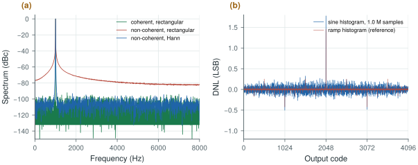
An FFT assumes that the record repeats forever. If the input completes a whole number of cycles in the record, it does, and the tone falls into one bin. If it does not, the jump at the record’s end spreads the tone over every bin as leakage, and the skirts bury the harmonics and the noise floor (Figure 22.1a).
Coherent sampling avoids leakage by choosing the input frequency:
Co-prime cycles also make every sample fall at a different phase, so the codes visit as many levels as possible. In simulation coherence is free. On the bench it needs a signal generator locked to the converter’s clock, with enough frequency resolution to hit \(f_\mathrm{in}\) exactly.
When coherence is impossible, for example with a free-running generator or a real ECG, a window tapers the record’s ends. A Hann window brings the leakage of a non-coherent tone from −80 dBc at a few hundred hertz away down below the 12-bit noise floor, at the price of spreading the tone over three bins and widening the noise bandwidth by 1.5. Sum the power of the bins under the main lobe for the signal, and exclude them from the noise. Close to the tone, though, the Hann sidelobes fall slowly: within a few tens of bins of a full-scale tone they still hold about −41 dBc, which caps the SNDR of an ideal 12-bit converter near 41 dB if only the main lobe is excluded. Exclude about 30 bins either side, or use a four-term Blackman–Harris window, whose leakage stays below the 12-bit floor outside its main lobe (Lab 6).
Try it below with an ideal converter: a 4096-point record, a tone of 67 cycles (prime, so coherent) and 12 bits. Slide the tone to 67.3 cycles, read the SNR, then add a window.
22.2FFT-based SNDR and SFDR
With the bins sorted into signal, harmonics, DC and noise, SNDR, SNR, THD and SFDR follow as in Chapter 14. Three practical points:
- Processing gain. The quantisation noise is spread over \(N_\mathrm{FFT}/2\) bins, so the noise floor per bin sits \(10\log_{10}(N_\mathrm{FFT}/2)\) dB below the total. A 4096-point FFT of an ideal 12-bit converter shows a floor near −107 dBc per bin, although the SNR is 74 dB. Do not read SNR from the height of the floor.
- Harmonics alias. In a sampled record the \(k\)-th harmonic lands at \(\lvert kf_\mathrm{in} - mf_\mathrm{s}\rvert\), often far from \(kf_\mathrm{in}\). Find each harmonic’s bin with
biosig.alias_freq(). - The source must be cleaner than the converter. A generator’s own harmonics and noise appear in the measurement. For 12 bits, filter the source with a passive band-pass filter at \(f_\mathrm{in}\); for 16 bits, use a dedicated low-distortion source.
22.3Histogram and ramp tests
The code-density (histogram) test measures DNL directly. With a slow linear ramp every code should be hit equally often; a wide code collects more hits. Ramps are hard to make linear on the bench. A sine wave is easy to make pure, but its codes are not equally likely: the input spends more time near the peaks. The expected fraction of hits for code \(k\) is the arcsine distribution:
\[p_k = \frac{1}{\pi}\left[\arcsin\frac{V_{k+1}}{A} - \arcsin\frac{V_k}{A}\right],\]and \(\mathrm{DNL}_k = h_k/(p_k N_\mathrm{samples}) - 1\). Slightly overdrive the converter, so that every code is reached, and estimate the amplitude and offset from the counts at the ends.
figsrc/ch22_figs.py applies a sine-wave histogram to the mismatched 12-bit SAR of Worked Example 14.1 and compares it with the ramp histogram (Figure 22.1b). With \(2^{20}\) samples, about 160 hits fall on each mid-scale code. Counting statistics give each DNL value a random error of \(1/\sqrt{160} = 0.079\) LSB; the simulated difference between the two methods is 0.071 LSB rms. Both find the mid-scale step of +1.45 LSB (the sine histogram reads 1.77 there, within its noise).
For a DNL resolution of 0.05 LSB you need about 400 hits per code. A sine crosses mid-scale fastest, so the middle codes collect the fewest hits and set the total: \(400\pi \cdot 2^{11} \approx 2.6\) million samples for 12 bits. At 16 kS/s that is under three minutes of data.
figsrc/ch22_figs.py.22.4Models versus transistors
A transistor-level simulation of a full SAR conversion takes seconds to minutes; an FFT test needs thousands of conversions; a system study needs millions. Behavioural models fill the gap: a Python or Verilog-A converter whose comparator has the simulated offset and noise, whose DAC has the extracted capacitor weights, and whose sampler has the simulated \(kT/C\) noise and droop. Lab 6’s adctest.py and the behavioural SAR of Chapter 18 are such models.
A model is useful only if it has been checked. Validate it at the transistor level at a few points, such as a handful of input levels for the static curve and one short coherent record for the spectrum, and compare the same metrics with the same code. Once they agree, use the model for everything that needs long records: histograms, Monte Carlo over mismatch, and the system simulations of Chapter 29.
22.5Testing a returned die
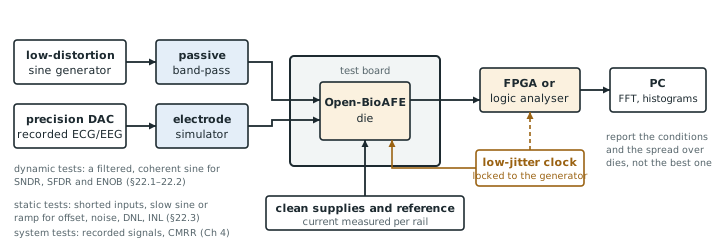
An OpenMPW die arrives months after tape-out with a few dozen pins and no second chance. Plan the bench before tape-out (Chapter 30; Figure 22.2):
- Power and bias first. Measure each supply’s current against simulation, with the converters idle and running.
- Static tests. Short the inputs and record the output codes: offset and noise (the code histogram’s width). Then a slow sine or ramp for the histogram DNL and INL.
- Dynamic tests. A filtered, coherent sine near full scale for SNDR, SFDR and ENOB, at several input frequencies across the band, and the converter’s power at the same time for the figure of merit.
- System tests. The whole channel with a recorded ECG or EEG played through a precision DAC and an electrode simulator (the imbalance network of Chapter 4), including the CMRR test.
- Report honestly. State the conditions (supply, temperature, clock, input frequency and amplitude, record length, window) with every number, and report the distribution over the dies measured, not the best one.
Use coherent sampling wherever you can, and a window where you cannot. Read SNR from the summed noise, not from the floor’s height, and find the harmonics where they alias. Measure DNL with a slightly overdriven sine and enough samples: about 400 hits per code for 0.05 LSB. Validate a behavioural model at a few transistor-level points, then use it for the long runs. Plan the bench, and the pins it needs, before tape-out.
Verification: coherent FFT (4096–65 536 points) for SNDR, SFDR and ENOB of both converters at the transistor level and with validated behavioural models; sine-histogram DNL/INL with at least \(2^{22}\) samples for the SAR; system tests with recorded ECG and EEG through an electrode simulator. Bench: precision DAC source, passive band-pass filters at the test frequencies, and a test mode that exposes each converter’s raw output.
Testing a ΔΣ modulator’s output with a plain Hann window and a short record. The strongly shaped out-of-band noise leaks back into the band through the window’s sidelobes and makes a good modulator look bad, as Chapter 19 found above 100 dB. Use a window with faster-falling sidelobes, a long record, or measure after the decimation filter.
Lab 6 builds adctest.py: coherent sampling, windows, SNDR, SFDR and ENOB, and histogram DNL/INL with injected capacitor mismatch. Check it against figsrc/ch22_figs.py, then reduce the record to \(2^{16}\) samples and watch the DNL estimate degrade.
Read with this chapter. Pelgrom [9] (characterisation of converters), Schreier, Temes and Pavan [10] (measuring ΔΣ modulators).
- Coherent sampling (\(f_\mathrm{in} = Mf_\mathrm{s}/N\), \(M\) odd) puts the tone in one bin; otherwise a window controls the leakage.
- The noise floor per bin is \(10\log_{10}(N/2)\) dB below the total; harmonics alias.
- Sine-histogram DNL needs the arcsine correction and enough hits: the error per code is \(1/\sqrt{\text{hits}}\), 0.08 LSB with 160 hits.
- Validated behavioural models carry the long and statistical runs; the transistor level checks them at a few points.
- Plan a returned die’s bench before tape-out: power, static, dynamic, system tests, with honest reporting.