Chapter 2Bioelectric Signals
Biopotentials range from microvolts to millivolts and from below one hertz to several kilohertz; this chapter measures them so that every later budget starts from real numbers.
- explain how an action potential arises, using the Hodgkin–Huxley model;
- describe the ECG waveform, its leads and Einthoven’s triangle;
- name the EEG bands and the 10–20 electrode system;
- tell surface EMG from needle EMG, and spikes from local field potentials and ECoG;
- compute the dynamic range and bandwidth the front-end has to handle.
What dynamic range and bandwidth must the Open-BioAFE signal chain handle?
2.1Action potentials
Every signal in this chapter starts at a cell membrane. A neuron or muscle cell keeps a different mix of ions inside and outside: more potassium inside, more sodium outside. Ion channels in the membrane let each ion leak through, and the concentration difference pulls it one way while the voltage it builds up pushes it back. The voltage at which the two balance is the ion’s Nernst potential.
At body temperature, 310 K, \(kT/q = 26.7\) mV. A mammalian neuron has about 140 mM of potassium inside and 5 mM outside, so \(E_\mathrm{K} = 26.7 \ln(5/140) \approx -89\) mV. Sodium, with about 12 mM inside and 145 mM outside, gives \(E_\mathrm{Na} \approx +67\) mV. The resting membrane sits between the two, close to \(E_\mathrm{K}\), because at rest far more potassium channels are open.
An action potential is what happens when the membrane is pushed above a threshold. Hodgkin and Huxley described it with four differential equations fitted to the squid giant axon [35], and Figure 2.1 solves their model. Sodium channels open first and the membrane swings towards \(E_\mathrm{Na}\); within a millisecond they close again and potassium channels open, pulling the voltage back down and slightly past rest. The whole event lasts one to two milliseconds and is about 100 mV tall.
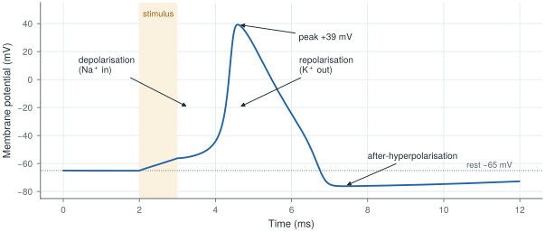
biosig.hodgkin_huxley().An electrode never sees this 100 mV directly, because it sits outside the cell. What reaches it is the small voltage that the membrane currents create as they flow through the surrounding tissue, summed over all the cells nearby and attenuated with distance. That is why the signals below are microvolts to millivolts, and why their size depends so much on where the electrode is.
2.2The electrocardiogram
The heart is a large, synchronised group of muscle cells, so its activity is the strongest biopotential on the body surface. Each beat starts in the sinoatrial node, spreads over the atria, pauses at the atrioventricular node, and then sweeps through the ventricles. Each phase leaves its mark on the electrocardiogram (ECG) (Figure 2.2): the P wave is atrial depolarisation, the QRS complex (about 80–100 ms) is ventricular depolarisation, and the T wave is ventricular repolarisation. At the skin the QRS is about a millivolt.
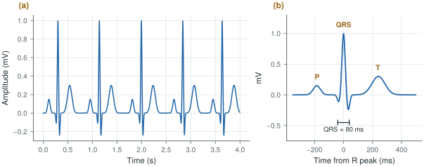
biosig.ecg()); real recordings come from PhysioNet in Lab 1.A lead is the voltage between two electrodes (or between one electrode and an average of others). Einthoven’s three limb leads use the right arm (RA), left arm (LA) and left leg (LL): lead I is LA − RA, lead II is LL − RA, and lead III is LL − LA, so that II = I + III. These three electrodes form Einthoven’s triangle. A clinical 12-lead ECG adds three augmented limb leads and six chest leads, from ten electrodes in total. A patch or a Holter records fewer leads, but each is still a differential voltage between two electrodes, which is why the front-end is a differential amplifier.
The bandwidth depends on the use. Diagnostic ECG keeps 0.05–150 Hz: the low corner is low enough not to distort the slow ST segment that indicates ischaemia, and the high corner keeps the sharp edges of the QRS. Monitoring ECG often uses 0.5–40 Hz to suppress baseline wander and muscle noise. Heart rates of 40 to 200 beats per minute put the fundamental between 0.7 and 3.3 Hz.
2.3The electroencephalogram
The electroencephalogram (EEG) is the summed activity of millions of cortical neurons, seen through the skull and scalp. The currents that add up are mostly the slow post-synaptic currents of pyramidal cells that point the same way, not the action potentials themselves [36]. After the skull has smeared and attenuated them, a few to a few hundred microvolts remain, typically tens of microvolts.
EEG is described by its rhythms, in five bands: δ (0.5–4 Hz, deep sleep), θ (4–8 Hz), α (8–13 Hz, relaxed with eyes closed), β (13–30 Hz, active thinking) and γ (30–100 Hz). The spectrum falls roughly as \(1/f\), with a peak where a rhythm is present (Figure 2.3). Electrodes are placed with the 10–20 system: positions at 10 % and 20 % of the distances between landmarks on the skull, 21 electrodes in the standard montage, with names such as Fz, Cz, O1 that encode the region and the side.
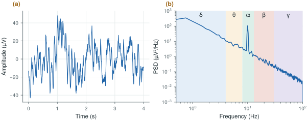
biosig.eeg().EEG sets the noise floor of the whole chip. A 10 µV rhythm measured over a 1.5 µVrms floor gives only 16.5 dB of signal-to-noise ratio, and the amplifier’s own \(1/f\) noise is largest exactly in the δ and θ bands. This is why Open-BioAFE uses chopping (Chapter 9).
2.4The electromyogram
A muscle is driven by motor neurons, and each motor neuron with the muscle fibres it controls forms a motor unit. When a motor unit fires, all its fibres produce an action potential together, and the electrode sees a motor-unit action potential. A stronger contraction recruits more motor units and fires them faster. Surface EMG is the sum of many such units seen through the skin (Figure 2.4a): it looks like noise whose envelope follows the force, reaches a few millivolts, and holds most of its power between about 20 and 150 Hz within a 10–500 Hz band. Needle EMG places the electrode inside the muscle and sees individual motor units, with sharper waveforms and a bandwidth of several kilohertz.
For prosthetic control, the useful information is the envelope and its pattern across channels, so the front-end needs bandwidth and dynamic range more than ultra-low noise: EMG is about a hundred times larger than EEG.
2.5Spikes, local field potentials and ECoG
An electrode inside the brain, within about 100 µm of a neuron, sees that neuron’s action potentials as spikes: biphasic pulses of 50–500 µV that last about a millisecond, in a band of roughly 300 Hz to 7 kHz (Figure 2.4b). The same electrode also picks up the local field potential (LFP), the summed slower currents of the surrounding tissue, below about 300 Hz. Electrocorticography (ECoG) places electrodes on the surface of the cortex, under the skull: its signals are larger and wider in bandwidth than scalp EEG because the skull is no longer in the way. Scalp EEG is the far end of the same chain [36].
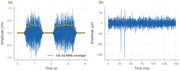
biosig.emg() and biosig.spikes().Spike recording is an optional mode for Open-BioAFE: its 7 kHz bandwidth and 20 kS/s or more per channel change the converter and the data rate (Chapter 1), but not the circuits of the front-end.
2.6Amplitude, bandwidth and dynamic range
Table 2.1 gathers the signals in one place, and Figure 2.5 draws each one as a box in amplitude and frequency. The same numbers are in SIGNALS in labs/python/biosig.py. Sources differ by a factor of a few, so treat them as design ranges, not limits.
Table 2.1. Amplitude and bandwidth of the main biopotentials. Typical ranges at the electrode, and a typical sample rate.
| Signal | Amplitude | Band | Typical sample rate |
|---|---|---|---|
| ECG (surface) | 0.5–4 mV | 0.05–150 Hz | 500 S/s |
| EEG (scalp) | 5–300 µV | 0.5–100 Hz | 256 S/s |
| EMG (surface) | 50 µV–5 mV | 10–500 Hz | 2 kS/s |
| EOG (eye movement) | 10 µV–3.5 mV | 0.05–50 Hz | 250 S/s |
| ECoG | 10–500 µV | 0.5–500 Hz | 2 kS/s |
| LFP (intracortical) | 50 µV–2 mV | 0.5–300 Hz | 1 kS/s |
| Spikes (extracellular) | 50–500 µV | 300 Hz–7 kHz | 30 kS/s |
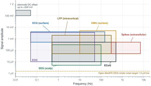
Two numbers in the figure dominate the design. The largest voltage at the input is not a signal at all but the electrode offset, up to ±300 mV (Chapter 3). The smallest is the noise target, 1.5 µVrms. The ratio between the largest input you must accept and the noise floor is the dynamic range, and it sets the number of bits. An ideal \(N\)-bit converter driven by a full-scale sine has a signal-to-quantisation-noise ratio of
A DC-coupled ECG or EEG channel must accept the full ±300 mV offset. A full-scale sine of 300 mV peak has an rms value of \(0.3/\sqrt{2} = 212\) mV. Over the 1.5 µVrms noise floor:
\[\mathrm{DR} = 20\log_{10}\frac{212\ \text{mV}}{1.5\ \text{µV}} \approx 103\ \text{dB}, \qquad N = \frac{103 - 1.76}{6.02} \approx 16.8\ \text{bits}\]That is more than a 16-bit converter gives (98 dB ideal). A 16-bit LSB over ±300 mV is 9.2 µV, and its quantisation noise, \(\mathrm{LSB}/\sqrt{12} \approx 2.6\) µVrms, is already above the noise target.
If the offset is blocked before the converter, the largest input is the signal itself. Surface EMG reaches about 5 mV peak, or 3.54 mVrms. Over 1.5 µVrms:
\[\mathrm{DR} = 20\log_{10}\frac{3.54\ \text{mV}}{1.5\ \text{µV}} \approx 67\ \text{dB}, \qquad N \approx 10.9\ \text{bits}\]EMG mode also integrates noise over a wider band (10–500 Hz instead of 0.5–100 Hz), so its noise floor is about \(\sqrt{490/99.5} \approx 2.2\) times higher and the need drops to about 60 dB, or 10 bits. A 12-bit SAR leaves margin.
The electrode offset, not the signal, sets the dynamic range of a DC-coupled chain. Open-BioAFE removes most of the offset in the front-end with a DC servo loop (Chapter 10), so that the gain stages do not saturate, and gives the ECG/EEG channel a 16-bit incremental ΔΣ for the remaining offset, artefacts and margin. The EMG and spike channels, AC-coupled, need only the 12-bit SAR.
Signal band 0.5 Hz–1 kHz (spike mode to 7 kHz optional); input-referred noise below 1.5 µVrms from 0.5 to 100 Hz in EEG mode; ±300 mV electrode offset tolerated.
Amplitudes in the literature are usually peak-to-peak or peak; noise is quoted in rms. A sine’s peak-to-peak value is \(2\sqrt{2}\) times its rms (9 dB), and the peak-to-peak value of Gaussian noise is often taken as about 6.6 times its rms. Mixing the two conventions can cost you 10–15 dB of dynamic range without anyone noticing. Always write which one a number is.
Lab 1 loads real ECG, EEG and EMG recordings from PhysioNet [5] and NinaPro [6], plots their traces and spectra, and measures their amplitude and bandwidth with the helpers in biosig.py. The result is your own version of Table 2.1.
Read with this chapter. Webster [7] for the physiology and the clinical bands, Buzsáki, Anastassiou and Koch [36] for where EEG, ECoG, LFPs and spikes come from.
- Biopotentials come from ionic currents across cell membranes; an electrode sees the small voltage these currents create in the tissue, summed and attenuated with distance.
- ECG is about 1 mV in 0.05–150 Hz; EEG is tens of microvolts in 0.5–100 Hz; surface EMG reaches a few millivolts in 10–500 Hz; spikes are 50–500 µV in 300 Hz–7 kHz.
- EEG sets the noise floor (1.5 µVrms); the electrode offset (±300 mV) sets the largest input.
- A DC-coupled chain needs about 103 dB, or 16.8 bits; an AC-coupled EMG chain about 60–67 dB, or 10–11 bits.
- Quote amplitudes with their convention: peak, peak-to-peak or rms.