Chapter 6Noise and the Noise–Power Trade-off
Every microvolt of noise you remove costs current. The noise efficiency factor tells you how close a design is to the physical limit.
- compute thermal, flicker, shot and \(kT/C\) noise and refer them to the amplifier input;
- integrate a noise spectrum over the signal band with the right noise bandwidth;
- derive the noise efficiency factor (NEF) and the power efficiency factor (PEF) and use them to compare designs;
- explain why a weak-inversion differential pair cannot do better than \(\mathrm{NEF} = \sqrt2\,n\), and what current reuse buys;
- set a current budget per channel from the 1.5 µVrms noise target.
What is the minimum supply current that can meet the EEG-mode noise target, and how close to it can a real amplifier get?
Chapter 5 measured the noise of single SG13G2 transistors. This chapter turns those numbers into a budget: how much noise each source adds, how to add them over the signal band, and how much current a given noise level costs. The budget starts from Chapter 3: of the 1.5 µVrms allowed from 0.5 to 100 Hz, the electrodes take 0.34 µVrms (wet) or 1.20 µVrms (dry), leaving the amplifier 1.46 µVrms or 0.9 µVrms.
6.1Noise sources
Four kinds of noise appear in a biopotential front-end.
Thermal noise. Any resistance \(R\) at temperature \(T\) produces a white voltage noise of density \(4kTR\) (V²/Hz). The electrode’s real part is one such resistance (Chapter 3); bias resistors and the channel of a MOSFET are others.
Shot noise. A current made of independent charges crossing a barrier fluctuates with density \(2qI\) (A²/Hz). The base current of a bipolar transistor carries it (Chapter 5), as does the leakage of a protection diode. In weak inversion, a MOSFET’s channel current is itself a diffusion current over a barrier, so its “thermal” noise is shot noise. Refer \(2qI_\mathrm{D}\) to the gate through \(g_\mathrm{m} = I_\mathrm{D}/(nU_T)\):
\[\overline{v_n^2} = \frac{2qI_\mathrm{D}}{g_\mathrm{m}^2} = \frac{2n^2 kT\,U_T}{I_\mathrm{D}} = \frac{2nkT}{g_\mathrm{m}},\]the expression Chapter 5 checked against the SG13G2 simulation (18.4 against 18.5 nV/√Hz at 1 µA). In strong inversion the factor \(n/2\) becomes about \(2/3\).
Flicker noise. The \(1/f\) noise of MOSFETs, \(K/(WLf)\), with \(K = 1.6\times10^{-10}\) V²·µm² for the SG13G2 low-voltage NMOS and \(5.4\times10^{-10}\) for the PMOS.
kT/C noise. A capacitor sampled through a switch keeps the switch’s thermal noise as a frozen voltage of variance \(kT/C\), whatever the switch resistance. On 1 pF that is 64 µVrms, spread from DC to half the sample rate. It sets the capacitor sizes of the converters (Chapter 14, Chapter 15) and of switched-capacitor filters (Chapter 11); oversampling divides its in-band part by the OSR.
6.2Input-referred noise and noise bandwidth
Noise is measured at the output but compared with the signal at the input. Divide the output noise density by the squared gain at each frequency to get the input-referred density, and integrate that over the band:
\[V_\mathrm{ni,rms}^2 = \int_0^\infty \overline{v_{ni}^2}(f)\,\lvert H(f)\rvert^2\,df,\]where \(H\) is the normalised shape of the band. For white noise only the area under \(\lvert H\rvert^2\) matters. That area is the noise bandwidth \(B_n\):
A first-order roll-off at 100 Hz lets through 57 % more white-noise power than an ideal brick wall at 100 Hz. Flicker noise behaves differently: each decade of frequency contributes the same power, so the ratio of the band edges decides it, and the shape of the roll-off hardly matters.
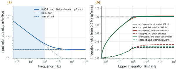
Take the NMOS pair of Chapter 5: 1800 µm² per device, 1 µA each, thermal floor \(\sqrt2 \times 18.5 = 26\) nV/√Hz.
Chopped (flicker noise removed, thermal only): a brick wall from 0.5 to 100 Hz gives \(26\ \text{nV} \times \sqrt{99.5} = 0.26\) µVrms; a first-order low-pass at 100 Hz gives 0.33 µVrms; a second-order Butterworth 0.28 µVrms (Figure 6.1b).
Unchopped: the flicker noise of the pair, \(\sqrt{2K\ln(200)/1800\ \text{µm}^2}\), dominates, and all three filter shapes give 1.00–1.02 µVrms. Moving the high-pass corner instead matters: the diagnostic ECG band of 0.05–150 Hz has \(\ln(3000) = 8.0\) instead of \(\ln(200) = 5.3\), which raises the flicker noise by 23 %.
With a real electrode the amplifier’s noise is not the whole story. An amplifier has a voltage noise \(e_n\) and a current noise \(i_n\), and the current noise flows through the electrode impedance. Together with the electrode’s own thermal noise the input sees
\[\overline{v_\mathrm{total}^2} = e_n^2 + i_n^2\,\lvert Z_\mathrm{e}\rvert^2 + 4kT\,\mathrm{Re}\{Z_\mathrm{e}\} \ \text{per hertz}.\]Above \(\lvert Z_\mathrm{e}\rvert = e_n/i_n\) the current noise dominates. For the SG13G2 HBT at 1 µA that crossover is \(15.1\ \text{nV}/21.6\ \text{fA} = 0.7\) MΩ, between a wet and a dry electrode, which is the trade-off of Figure 5.3. A MOSFET’s gate current is so small that its current noise matters only for implanted microelectrodes.
6.3Noise efficiency factor and power efficiency factor
Noise can always be lowered by spending more current, so a noise number alone says little about a design. Steyaert and Sansen [14] normalised it by the current with the noise efficiency factor, and Harrison and Charles [15] made it the standard yardstick for neural and biopotential amplifiers:
\(I_\mathrm{tot}\) is the total supply current of the amplifier and BW its −3 dB bandwidth; the \(\pi/2\) inside assumes the noise rolls off with one pole, so that \(B_n = (\pi/2)\,\mathrm{BW}\). For a band that is cut sharply by a digital filter afterwards, as in Open-BioAFE, use \(\mathrm{BW} = 2B_n/\pi\). The definition can then be turned around into a current budget:
\[I_\mathrm{tot} = \mathrm{NEF}^2\,\frac{4kT\,U_T\,B_n}{V_\mathrm{ni,rms}^2}.\]The power efficiency factor multiplies by the supply voltage, so that a design at 1.2 V and one at 3.3 V can be compared on power rather than current.
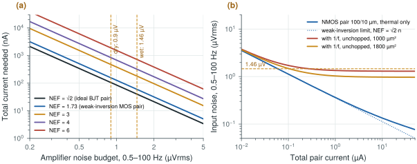
With \(B_n = 99.5\) Hz, \(4kT\,U_T\,B_n = 4.26\times10^{-20}\) A·V². For the wet-electrode budget of 1.46 µVrms:
- an amplifier at the weak-inversion limit, \(\mathrm{NEF} = 1.73\) (section 6.4), needs 60 nA;
- a good real amplifier at NEF 3 needs 180 nA, and one at NEF 4 needs 320 nA.
For the dry-electrode budget of 0.9 µVrms the same amplifiers need 157 nA, 474 nA and 842 nA (Figure 6.2a). At 1.2 V, NEF 3 is a PEF of 10.8.
These currents are tiny next to the 8 µA a 10 µW channel can draw. Thermal noise alone does not explain why biopotential amplifiers spend microamperes. Figure 6.2b shows the first reason: without chopping, the flicker noise of a realistically sized pair is a floor that no current can push down. A 1000 µm² pair stays at 1.3 µVrms however much current it gets. The others are bandwidth (a chopped amplifier must amplify at the chopping frequency, kilohertz rather than hertz), the noise of every device after the input pair, and the extra stages that set gain, offset rejection and input impedance.
The demo below draws the same equation for any band, current and NEF. The dashed lines are amplifiers at NEF 1.73, 3 and 6; the dot is yours.
6.4The physical limit
How low can the NEF go? Consider a differential pair whose only noise is that of its two input transistors, each carrying half of \(I_\mathrm{tot}\). For ideal bipolar transistors, each contributes \(2kT/g_\mathrm{m}\) with \(g_\mathrm{m} = I_\mathrm{tot}/(2U_T)\), and the pair’s input noise is the sum of the two:
\[\overline{v_{ni}^2} = 2 \times \frac{2kT \cdot 2U_T}{I_\mathrm{tot}} = \frac{8kT\,U_T}{I_\mathrm{tot}}.\]Put this into the current-budget form of the NEF and the pair gives \(\mathrm{NEF}^2 = 8/4 = 2\), or NEF = √2. A weak-inversion MOS pair has \(n\) times less \(g_\mathrm{m}\) per microampere, which multiplies the noise power by \(n^2\):
The SG13G2 NMOS pair of Figure 6.2b reaches 1.72 at 100 nA, and 2.05 at 10 µA where its devices drift into moderate inversion. A real amplifier adds the noise of its other transistors. In a simple OTA the current-mirror load adds power in proportion to \(g_\mathrm{m,load}/g_\mathrm{m,in}\): with loads in strong inversion at 5 V⁻¹ and inputs at 30 V⁻¹ that is 17 % more power, or 8 % more NEF. Cascodes, folding branches and bias circuits add more. Published capacitive-feedback amplifiers sit around NEF 2–4; the original design of Harrison and Charles reached 4.0 [15].
One trick goes below \(\sqrt2\,n\). If the same current flows through an NMOS and a PMOS that both see the input, as in an inverter-based or complementary input stage, the two transconductances add while the current is spent once. The input noise power halves, and the limit falls to about \(n \approx 1.2\). This current reuse comes at a price in SG13G2: the PMOS adds its larger flicker noise and its excess thermal noise (Chapter 5), so it pays off only in a chopped amplifier at a supply high enough to stack the two devices.
Give the first stage 2 µA, a quarter of the channel’s budget. At NEF 3, its thermal noise over 0.5–100 Hz is
\[V_\mathrm{ni} = 3\sqrt{\frac{4.26\times10^{-20}}{2\ \text{µA}}} = 0.44\ \text{µVrms},\]half the dry-electrode budget, provided chopping removes the flicker noise. Added in power to the dry electrodes’ 1.20 µVrms, the channel totals \(\sqrt{1.20^2 + 0.44^2} = 1.28\) µVrms, within the 1.5 µVrms target with room for the later stages.
The thermal-noise floor costs well under a microampere at the EEG target; a weak-inversion MOS pair cannot beat NEF 1.73, and a good amplifier reaches 3. Spend the rest of the budget on what thermal-noise arithmetic ignores: removing flicker noise (chopping), amplifying at the chopping frequency, and the later stages. Judge every design by its NEF and PEF, compute noise over the real band edges, and remember that a first-order roll-off adds 57 % of white-noise power.
First stage: about 2 µA from 1.2 V, NEF ≤ 3 (PEF ≤ 11), thermal noise ≤ 0.45 µVrms over 0.5–100 Hz, flicker noise removed by chopping (Chapter 9). Whole channel with dry electrodes: about 1.3 µVrms against the 1.5 µVrms target.
NEF values are only comparable when they use the same bandwidth convention. The definition assumes a first-order roll-off with BW its −3 dB frequency; quoting the NEF of a brick-wall band with BW set to the band width makes an amplifier look \(\sqrt{\pi/2} = 1.25\) times better than it is. Also check that \(I_\mathrm{tot}\) includes the bias circuits and, for chopped amplifiers, the clock drivers.
Lab 4 computes the NEF of your Harrison LNA versus bias current. Before building it, reproduce Figure 6.2b from figsrc/data/sg13_gmid.csv: it tells you the best NEF your input pair can reach at each current.
Read with this chapter. Steyaert and Sansen [14], Harrison and Charles [15], Sarpeshkar [12] (noise in subthreshold circuits), Razavi [13] (the chapter on noise).
- Thermal noise \(4kTR\), shot noise \(2qI\), flicker noise \(K/(WLf)\) and \(kT/C\); in weak inversion a MOSFET’s channel noise is the shot noise of its current, \(2nkT/g_\mathrm{m}\) at the gate.
- White noise integrates over the noise bandwidth (\(\pi/2\) times the corner for one pole); flicker noise over \(\ln(f_\mathrm{H}/f_\mathrm{L})\), so only the band edges matter.
- NEF normalises noise by current; with a brick-wall band, \(I_\mathrm{tot} = \mathrm{NEF}^2\,4kTU_TB_n/V_\mathrm{ni}^2\).
- A weak-inversion MOS pair cannot beat NEF \(\sqrt2\,n = 1.73\) in SG13G2; current reuse can approach \(n\).
- The EEG target needs only 60–840 nA of thermal-noise current; flicker noise, chopping bandwidth and later stages are what cost microamperes.