Chapter 24ECG Processing
Detecting heartbeats is the oldest biomedical DSP problem, and the best way to see how ADC bits and amplifier noise reach a clinical result.
- implement the Pan–Tompkins QRS detector;
- compute heart rate and heart-rate variability metrics;
- classify beats on the MIT-BIH Arrhythmia Database;
- test robustness with the MIT-BIH Noise Stress Test Database;
- show how ADC bits and AFE noise move detection sensitivity;
- estimate what detection on the chip costs and what it saves.
How many bits and how much input noise can the ECG chain afford before QRS detection degrades?
Everything an ECG system reports, heart rate, rhythm, arrhythmia alarms, starts with finding each QRS complex. This chapter builds the standard detector, uses it to answer the design question with a behavioural model of the Open-BioAFE chain, sketches what comes after detection, and counts what detection costs on the chip. The figures use the synthetic ECG of biosig.ecg(), whose beat times are known exactly; Lab 11 repeats the study on real recordings.
24.1Pan–Tompkins QRS detection
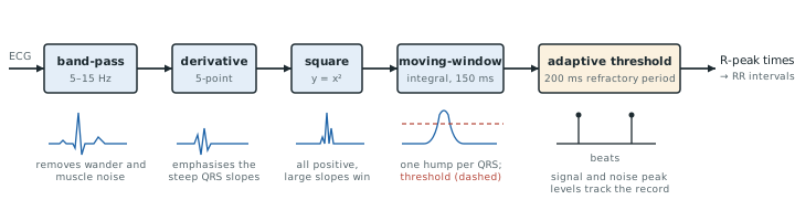
The detector of Pan and Tompkins [29] has stayed the reference for four decades because each of its stages has a clear job (Figure 24.1):
- a band-pass filter at 5–15 Hz keeps the QRS energy and rejects baseline wander, P and T waves, and muscle noise;
- a derivative emphasises the QRS’s steep slopes;
- squaring makes everything positive and stresses large slopes over small ones;
- a moving-window integrator of about 150 ms, the width of a wide QRS, turns each complex into one smooth pulse;
- adaptive thresholds, which track running estimates of the signal-peak and noise-peak levels, decide which pulses are beats, with a 200 ms refractory period after each one.
The original stages are integer recursions for 200 S/s, and the only multiplication is the square:
The low-pass, two 6-sample running sums with a first zero at 33 Hz and a gain of 36, and the high-pass, a 16-sample delay minus a 32-sample average, together pass 4.9–11.8 Hz at −3 dB; with the derivative, 6.6–14.6 Hz, where the QRS has its energy and the P and T waves have little (Figure 24.2b). An integrator peak \(P\) above THR is a beat, and the one-eighth updates forget an old level with a time constant of about eight peaks. The full algorithm adds a search back with a lower threshold and a slope test against T waves [29]; the compact versions in this chapter omit both.
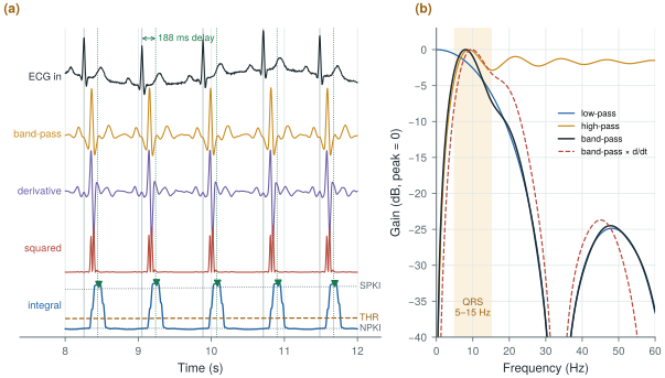
figsrc/ch24_figs.py.The integral’s broad peak scatters by 3 ms rms in Figure 24.2a, 8.5 ms with 50 µVrms of noise, so it only says that a beat occurred; the R peak is then found on the band-passed signal within ±75 ms.
Rescale the filters to keep their time spans. Their group delays at 10 Hz are:
- 200 S/s: low-pass 5 samples, high-pass 16.1, derivative 2, 30-sample integrator 14.5; in total 37.6 samples, 188 ms;
- 500 S/s: 15- and 80-sample filters and a \(0.15 \times 500 = 75\)-sample window; \(14 + 40.1 + 2 + 37 = 93.1\) samples, 186 ms;
- 250 S/s, the on-chip detector’s rate: a 38-sample window (37.5 rounded) and 190 ms.
The delay is fixed by the time spans, about 0.19 s at any rate. The rate sets the memory, 81 words at 200 S/s and 192 at 500 S/s, and the work (Worked Example 24.4). With the QRS band ending near 15 Hz, a faster rate does not help detection: in the runs of Figure 24.3c every beat is found at every rate from 100 to 500 S/s.
The original paper reported detecting 99.3 % of the beats in the MIT-BIH Arrhythmia Database [30]. figsrc/ch24_figs.py contains the integer version and a compact one with a Butterworth band-pass at 500 S/s, whose stages Figure 24.4a shows.
The demo below runs the detector of Figure 24.1 on a 20 s synthetic ECG with heart-rate variability, using the original integer filters at 200 S/s. Step through the stages, then add noise or take bits away and watch the sensitivity and positive predictivity.
24.2Heart rate and HRV
The intervals between successive R peaks, the RR intervals, give the instantaneous heart rate. Their variation, heart-rate variability, reflects the autonomic nervous system. Time-domain metrics are SDNN (the standard deviation of normal RR intervals) and RMSSD (the rms of successive differences). Frequency-domain metrics are the power in the low-frequency (0.04–0.15 Hz) and high-frequency (0.15–0.4 Hz) bands of the RR series, after resampling it to a uniform rate. HRV needs R-peak times accurate to a few milliseconds, which 500 S/s and a peak refinement on the band-passed signal provide; 125 S/s with parabolic interpolation of the peak is almost as good.
Only normal-to-normal (NN) intervals between sinus beats count, so ectopic, missed and false beats must be edited out first. RMSSD follows mainly the fast, respiratory (HF) variation; SDNN also includes the slow drifts. For the spectrum, the RR values are interpolated onto a uniform grid of a few hertz, or analysed directly with a Lomb–Scargle periodogram. The bands and the five-minute convention for short-term HRV follow the HRV task force [62].
The record of Figure 24.3 follows the two-peak RR spectrum of the McSharry model [37]: 0.1 and 0.25 Hz, LF:HF power 0.5, mean RR 800 ms, expected SDNN 50 ms. Its first eight intervals are 835, 821, 746, 717, 766, 843, 854 and 789 ms:
- the mean is 796.4 ms, so the heart rate is 75.3 beats per minute;
- the squared deviations sum to 17 408 ms², so \(\mathrm{SDNN} = \sqrt{17\,408/7} = 49.9\) ms;
- the successive differences, −14, −75, −29, +49, +77, +11 and −65 ms, have squares summing to 19 338 ms², so \(\mathrm{RMSSD} = \sqrt{19\,338/7} = 52.6\) ms.
The full five minutes (371 beats) give SDNN 45.2 ms, RMSSD 46.9 ms and LF/HF 0.32. Over 200 records from the same process, the middle 80 % of SDNN estimates spans 34–63 ms from one minute and 43–57 ms from five; LF/HF spans 0.16–2.6 and 0.27–1.1. One minute holds barely two cycles of 0.04 Hz: quote SDNN and RMSSD from a minute or two with error bars, LF/HF only from five minutes. The method matters too: interpolating onto the 4 Hz grid raised LF/HF by 11 % with a shape-preserving cubic and by 28 % with straight lines.
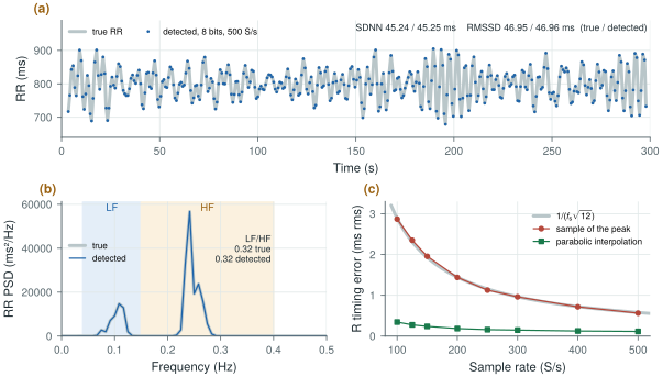
figsrc/ch24_figs.py.A timing error of \(\sigma_t\) rms per beat adds \(2\sigma_t^2\) to SDNN² and \(6\sigma_t^2\) to RMSSD², since \(\mathrm{RR}_{i+1} - \mathrm{RR}_i = t_{i+2} - 2t_{i+1} + t_i\). Taking the highest sample gives \(\sigma_t = 1/(f_\mathrm{s}\sqrt{12})\): 0.58 ms at 500 S/s, 2.3 ms at 125 S/s. A subject with little variability, an RMSSD of 10 ms, then reads 10.1 ms at 500 S/s but 11.5 ms at 125 S/s; with parabolic interpolation, 10.02 ms even at 125 S/s. Amplitude resolution hardly enters: at 8 bits the timing error is 0.12 ms rms.
HRV asks the converter for timing, not resolution: an 8-bit monitoring mode reproduces the HRV of the 16-bit chain. On Open-BioAFE, detect at the on-chip detector’s low rate, then place each R peak by parabolic interpolation on the 500 S/s stream, to about 0.1 ms. A 16-bit RR interval in 0.25 ms units spans 16 s and rounds by only 0.07 ms rms.
Computing HRV from unedited detections. In the record of Figure 24.3, deleting one beat of 371 raises RMSSD from 46.9 to 73.5 ms and SDNN from 45.2 to 61.6 ms; one false beat raises RMSSD to 56.0 ms. Reject intervals that differ from their neighbours by more than a set fraction, and report how many were removed.
24.3Beat classification
Once beats are found, each can be described by a handful of features: RR intervals before and after, QRS width, amplitudes, and a few coefficients of its shape. A simple classifier, from thresholds to linear discriminants, separates normal beats from ventricular ectopic beats with high accuracy on the MIT-BIH database. Two precautions keep the results honest. Train and test on different patients, because beats from the same patient look alike. And report sensitivity and positive predictivity per class, not overall accuracy, because normal beats dominate the database.
Detection and classification are scored alike: a detection within a fixed tolerance of a reference annotation is a true positive (TP), an unmatched annotation a false negative (FN), an unmatched detection a false positive (FP).
One missed beat in 70 gives Se = 69/70 = 98.6 %. Per class, a ventricular beat called normal is a false negative for the ventricular class; and if 2 % of the beats are ventricular, calling every beat normal is 98 % accurate with a ventricular sensitivity of zero.
24.4Noise stress testing
Real recordings carry baseline wander, muscle noise and electrode motion. The MIT-BIH Noise Stress Test Database [31] provides calibrated recordings of each noise type, to be added to clean ECG at chosen signal-to-noise ratios. Electrode-motion noise is the hardest, because its spectrum overlaps the QRS’s. A detector, or a front-end, is characterised by how its sensitivity and positive predictivity fall as the SNR drops. Lab 11 runs this test: electrode motion breaks the detector long before the bits or the front-end noise do.
24.5Co-design: bits and noise versus sensitivity
A behavioural chain answers the design question: synthetic ECG (1 mV R wave, 75 beats per minute with 5 % variability), plus white input noise, plus 200 µV of baseline wander, through a converter whose ±5 mV input range is quantised to \(B\) bits (a gain of 100 into the ±0.5 V converter of Part III), then the detector.
Over 70 beats (Figure 24.4b):
- with 5 bits or more and up to 100 µVrms of input noise, sensitivity and positive predictivity are both 100 %;
- with 200 µVrms of noise they stay at 98.6–100 %;
- with 4 bits, sensitivity falls to 85–96 %, and with 3 bits to about 50–60 %.
QRS detection is extraordinarily tolerant: five bits over ±5 mV is an LSB of 312 µV, and 100 µVrms is sixty-seven times the EEG noise target.
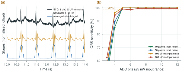
figsrc/ch24_figs.py.The lesson is not that the Open-BioAFE specification is too strict. Its 16 bits and 1.5 µVrms are set by EEG and by diagnostic ECG morphology, ST levels of tenths of a millivolt and P waves of a few tens of microvolts (Chapter 2). The lesson is that a heart-rate monitor could run the same chip in a much cheaper mode: a few bits, a relaxed front-end bias, a lower sample rate. HRV survives such a mode too (Section 24.2). That trade belongs in the system budget of Chapter 29.
24.6Detection on the chip
Detection takes a few additions per sample, so it can run on Open-BioAFE, which then needs to send only the beats (Chapter 27).
Work. As recursions, with power-of-two scalings as free shifts, the detector needs 15 operations per sample: 4 additions in the low-pass, 3 in the high-pass, 3 in the derivative, one squaring, 2 in the integrator and 2 peak comparisons. That is 3750 per second per channel at 250 S/s and 7500 at 500 S/s; eight channels at 500 S/s take 11.7 % of one operation per cycle of the 512 kHz feature clock (Chapter 29). At an assumed 1 pJ per operation, an order of magnitude for synthesis to replace (Chapter 30), that is 7.5 nW per channel at 500 S/s, inside Chapter 29’s 0.3 µW per channel for features and decimation.
Multiplier. A 1 mV R wave uses 7.9 % of the derivative’s range. Rounding the derivative to its top 8, or even 6, bits before squaring still found every beat with 50 or 200 µVrms of noise: an 8 × 8-bit squarer is plenty.
Data. Raw ECG is 64 kb/s for eight channels. One 16-bit RR interval per beat is 20 b/s at 75 beats per minute (48 b/s at 180), 3200 times less. At Chapter 27’s 5 nJ per radio bit, raw ECG costs 320 µW, its 0.34 kb/s feature budget 1.7 µW, and the RR intervals alone 0.1 µW.
At such low activity, leakage may outweigh switching, one more reason to detect at 250 S/s with about half the memory. And no cardiologist can review a rhythm from beat times: keep the raw stream available on demand.
Size the chain for the most demanding use of the signal, not for the easiest. QRS detection works with 5 bits and 100 µVrms of noise, so a monitoring mode can save a great deal of power; diagnostic morphology and EEG set the full specification. Validate every claim on real recordings with noise added from the Noise Stress Test Database, and report sensitivity and positive predictivity, per class, on patients the detector was not tuned on. Put the detector on the chip: it costs nanowatts per channel and turns 64 kb/s of raw ECG into tens of bits per second.
On-chip QRS detection (Pan–Tompkins at 250 S/s) for heart rate and RR intervals in a low-power monitoring mode, each R peak placed by parabolic interpolation on the 500 S/s stream and sent as a 16-bit RR interval in 0.25 ms units; full 16-bit, 500 S/s raw ECG in diagnostic mode. A monitoring mode with the ΔΣ reduced to about 8 bits and the front-end bias halved is a candidate for the budgets of Chapter 29.
Scoring a detector on a different time window from the reference annotations. Detections in a stretch the reference does not cover count as false positives and lower the positive predictivity for no real reason; an early version of this chapter’s script did exactly that and reported 92 %. Score detections and annotations over the same window, with a fixed tolerance (75–150 ms).
Lab 11 runs MIT-BIH records and the Noise Stress Test through a behavioural front-end and ADC with Pan–Tompkins detection, and plots sensitivity and positive predictivity against ADC bits and input noise. Start from figsrc/ch24_figs.py, replace biosig.ecg() with a record loaded by wfdb, and add electrode-motion noise at 6, 0 and −6 dB SNR. Then compute HRV from the detections with hrv_time() and hrv_freq() and compare it with the annotations’ normal beats.
Read with this chapter. Pan and Tompkins [29], Tompkins [28], the HRV task force [62], McSharry et al. [37] for the synthetic ECG and RR model, the MIT-BIH Arrhythmia Database [30] and Noise Stress Test Database [31].
- Pan–Tompkins: 5–15 Hz band-pass, derivative, squaring, 150 ms integration, adaptive thresholds with a refractory period; about 190 ms of delay at any sample rate.
- RR intervals give heart rate and HRV (SDNN, RMSSD, LF/HF power). HRV needs edited normal-to-normal intervals and R timing of a millisecond or better, which parabolic interpolation gives from 100 to 500 S/s; LF/HF needs five minutes.
- Classify beats with patient-independent training, and score by sensitivity and positive predictivity per class.
- In a behavioural chain, QRS detection stays at 100 % with 5 bits over ±5 mV and up to 100 µVrms of noise, and HRV is unchanged at 8 bits.
- On the chip, detection takes 15 operations per sample and replaces 64 kb/s of raw ECG with about 20 b/s of RR intervals.
- The chip’s specification is set by EEG and diagnostic morphology; heart-rate monitoring could run in a far cheaper mode.