Chapter 9Chopper Stabilisation and Offset Cancellation
Chopping moves the signal above the flicker-noise corner, amplifies it there and brings it back, leaving the offset and \(1/f\) noise behind.
- explain chopping as modulation and demodulation in the frequency domain;
- predict the residual offset and the output ripple of a chopper amplifier;
- design a ripple-reduction loop;
- compare chopping, auto-zeroing and correlated double sampling;
- quantify the input-impedance cost of an input chopper.
How much offset, ripple and input-impedance loss does chopping leave behind, and how do you suppress each?
Chapters 5, 7 and 8 kept arriving at the same conclusion. Flicker noise in the EEG band forces input devices of thousands of square micrometres, the input pair’s offset of 0.1–0.4 mV is a hundred times the noise target, and the capacitively coupled IA’s own CMRR stops at about 78 dB. Chopping fixes all three. This chapter shows how, and what it costs.
9.1The modulation view of chopping
A chopper is four switches that either pass a differential signal straight through or cross it over, swapping the two wires. Driven by a clock at \(f_\mathrm{ch}\), it multiplies the signal by a square wave \(m(t) = \pm1\). Put one chopper at the amplifier’s input and an identical one at its output, and the signal is multiplied twice, \(m^2 = 1\): it passes through unchanged, apart from the amplifier’s gain. The amplifier’s own offset and flicker noise enter after the input chopper, so they are multiplied only once.
In the frequency domain, multiplying by a square wave copies a spectrum to the odd harmonics of \(f_\mathrm{ch}\), with weights \(4/(\pi k)\) for harmonic \(k\). The input chopper moves the biosignal from baseband up around \(f_\mathrm{ch}\), where the amplifier is quiet. The output chopper moves it back down. At the same time it moves the amplifier’s offset and \(1/f\) noise up to \(f_\mathrm{ch}\), where a low-pass filter removes them (Figure 9.1).
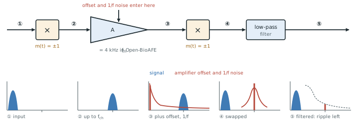
The baseband noise of a chopped amplifier is its white noise plus whatever flicker noise remains near \(f_\mathrm{ch}\) and its harmonics. If \(f_\mathrm{ch}\) is well above the flicker corner \(f_\mathrm{c}\), the remainder is small. The factor \(0.85 = (8/\pi^2)\sum_{k\ \mathrm{odd}} k^{-3}\) comes from summing the harmonics of the \(1/f\) part.
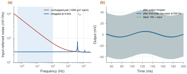
The 1000 µm² NMOS pair at 1 µA per device has a flicker corner of \(1.58\times10^{-13}/(18.5\ \text{nV})^2 = 460\) Hz. Unchopped, its noise over 0.5–100 Hz is 1.29 µVrms, nearly all flicker. Chopped at 4 kHz, the baseband spectrum is flat at the thermal floor (Figure 9.2a) and the noise falls to 0.273 µVrms, 5 % above the 0.26 µVrms thermal floor of the pair.
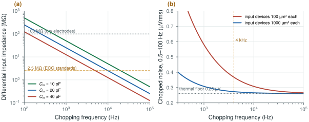
A 100 µm² pair has a corner of 4.6 kHz. Chopped at the same 4 kHz it gives 0.367 µVrms, 40 % above the floor; it needs about 10 kHz to come within 20 % (Figure 9.3b).
figsrc/ch09_figs.py.9.2Residual offset and ripple
Chopping does not make the offset vanish. It moves it, and it adds a small offset of its own.
Ripple. The amplifier’s offset, multiplied by the output chopper, becomes a square wave at \(f_\mathrm{ch}\) whose amplitude is the offset times the gain. For a 100 µm² pair, \(\sigma(V_\mathrm{os}) = 3.9/\sqrt{100} = 0.39\) mV, and at a gain of 100 the ripple is ±39 mV (Figure 9.2b). That is ten times the largest EEG at the output, and it eats a large part of the 1.2 V swing. A second-order low-pass filter at 200 Hz attenuates it by \((4000/200)^2 = 400\), to about 0.1 mV. Inside the amplifier, however, the ripple is still there, and its slewing and the following stage’s linear range must cope with it.
Residual offset. The input chopper’s switches inject charge on every transition. If the two halves inject slightly different charges \(\Delta q\), the mismatch flows through the source impedance \(R_\mathrm{s}\) twice per period, and the average current \(2f_\mathrm{ch}\Delta q\) produces a DC error:
\[V_\mathrm{os,res} \approx 2 f_\mathrm{ch}\,\Delta q\,R_\mathrm{s}.\]With \(\Delta q = 1\) fC and \(f_\mathrm{ch} = 4\) kHz, that is 0.4 µV for a 50 kΩ wet electrode but 8 µV for a 1 MΩ dry one. The residual offset grows with \(f_\mathrm{ch}\), so the chopping frequency should sit just above the flicker corner rather than as high as possible. Small, matched switches with dummy devices keep \(\Delta q\) low.
Clock errors. A chopper clock whose duty cycle is not exactly 50 %, or whose two phases overlap or leave a gap, demodulates the signal imperfectly: the effective gain drops and a residue of the ripple appears at baseband. Non-overlapping clocks with a short, well-defined gap and a symmetric layout keep this small. Synchronising the chopper clock with the converter’s sampling clock keeps the ripple and its harmonics from aliasing into the band (Chapter 13).
The demo below puts the two sections together. It starts at Open-BioAFE’s choice, 1000 µm² input devices (corner 460 Hz, 26 nV/√Hz) chopped at 4 kHz; switch the chopper off, slide fch below the corner, or move to dry electrodes and watch the residual offset.
9.3Ripple-reduction loops
Filtering the ripple after the amplifier works, but it leaves the ripple inside it. A ripple-reduction loop removes the offset at its source. It senses the ripple at the amplifier output, before the output chopper has turned the signal back to baseband, where the ripple is a square wave at \(f_\mathrm{ch}\) and the signal is still up-modulated. A third chopper demodulates the ripple to DC, an integrator accumulates it, and the result is fed back as a correction current into the amplifier’s first stage until the ripple disappears. The loop’s gain is high only at DC, so it nulls the static offset without touching the signal. The reference design of Yazicioglu et al. [17] combined a chopper, a ripple-reduction loop and a DC servo loop in a 60 µW ExG front-end with 60 nV/√Hz of input noise.
For Open-BioAFE, a ripple-reduction loop makes it possible to use small input devices (100 µm², 0.39 mV of offset) without ±39 mV of internal ripple. The alternative is larger input devices with less offset (1000 µm², 0.12 mV and ±12 mV of ripple) and a lower chopping frequency.
9.4Auto-zero and correlated double sampling
Auto-zeroing is the other classic way to remove offset and flicker noise. In one phase the amplifier’s inputs are shorted and its offset is sampled onto a capacitor; in the next phase the stored value is subtracted from the signal. Correlated double sampling does the same thing with two samples of the output per period. Both cancel offset and the slow part of the flicker noise well.
Their weakness is noise folding. Sampling the amplifier’s white noise, whose bandwidth \(f_\mathrm{n}\) is far above the sampling rate \(f_\mathrm{s}\), aliases all of it into the baseband, raising the white noise power by roughly \(2f_\mathrm{n}/f_\mathrm{s}\). For an amplifier with \(f_\mathrm{n} = 24\) kHz auto-zeroed at 4 kHz, that is a factor of about 12 in power, 3.5 in amplitude. Chopping is a continuous-time multiplication, folds nothing, and keeps the white noise at its floor. That is why biopotential front-ends chop, while auto-zeroing remains useful in sampled circuits such as the comparators of Chapter 16.
9.5Chopper spikes and input impedance
The input chopper has one serious cost. In a capacitively coupled IA it sits in front of the input capacitors, and on every transition it reverses the voltage across them. The electrode must supply the charge for that reversal twice per period, which looks like a resistor:
With \(C_\mathrm{in} = 20\) pF, the differential input impedance is 25 MΩ at 1 kHz, 6.25 MΩ at 4 kHz and 2.5 MΩ at 10 kHz (Figure 9.3a). At 10 kHz the amplifier just meets the 2.5 MΩ the ECG standards require (Chapter 3). At 4 kHz it has a margin of 2.5 over the standard, but it is sixteen times below the 100 MΩ that dry electrodes need. A 1 MΩ dry electrode in front of 6.25 MΩ loses 14 % of the signal and converts common mode into differential mode through any imbalance.
Every choice of chopping frequency is therefore a three-way trade. Higher \(f_\mathrm{ch}\) removes more flicker noise; lower \(f_\mathrm{ch}\) keeps the input impedance and the residual offset in check. The amplifier’s bandwidth must exceed \(f_\mathrm{ch}\) by a comfortable factor, which costs current. Chapter 10 restores the impedance with a positive-feedback boosting loop.
figsrc/ch09_figs.py.Chop the first stage just above its flicker corner. With 1000 µm² input devices that is about 4 kHz, which brings the noise to within 5 % of the thermal floor. Expect three costs and plan for each: a ripple of the offset times the gain at \(f_\mathrm{ch}\) (filter it or null it with a ripple-reduction loop), a residual offset of \(2f_\mathrm{ch}\Delta qR_\mathrm{s}\) (small switches, dummies, matched layout), and an input impedance of \(1/(2f_\mathrm{ch}C_\mathrm{in})\) (boost it, Chapter 10). Keep the chopper clock clean, non-overlapping and synchronous with the converter.
Chopping frequency 4 kHz, synchronous with the converter clock. Input pair 1000 µm² per device (for example \(W/L = 100/10\) µm), 1 µA each: chopped noise 0.27 µVrms over 0.5–100 Hz before the capacitive noise gain, about 0.31 µVrms after it. Offset ripple ±12 mV (1σ) at the LNA output, removed by a ripple-reduction loop or the following low-pass filter. Input impedance 6.25 MΩ before boosting.
Simulating a chopper amplifier only with AC and noise analyses. Chopping is a time-varying operation, so a plain .noise run shows the unchopped spectrum, and .ac misses the ripple, the residual offset and the input-impedance loss entirely. Use transient noise or periodic steady-state analysis, or at least a long transient with a small sine input, and measure the input current to get the true input impedance.
Lab 5 adds input and output choppers and a DC servo loop to your LNA: \(1/f\) removal, ripple, input-impedance loss and ±300 mV offset tolerance. Reproduce Figure 9.3b first with figsrc/ch09_figs.py, then compare it with a transient-noise simulation of your amplifier.
Read with this chapter. Yazicioglu et al. [17], Yazicioglu, Van Hoof and Puers [8].
- Two choppers pass the signal and move the amplifier’s offset and \(1/f\) noise to \(f_\mathrm{ch}\); the baseband noise approaches the white floor when \(f_\mathrm{ch}\) is above the flicker corner.
- For the 1000 µm² SG13G2 pair (corner 460 Hz), chopping at 4 kHz cuts the EEG-band noise from 1.29 to 0.27 µVrms.
- The offset becomes a ripple of offset × gain at \(f_\mathrm{ch}\) (±39 mV for a 100 µm² pair at gain 100); a ripple-reduction loop nulls it at its source.
- Charge-injection mismatch leaves \(2f_\mathrm{ch}\Delta qR_\mathrm{s}\) of residual offset, 0.4–8 µV for 1 fC at 4 kHz.
- Auto-zeroing folds wideband noise into the band; chopping does not.
- A chopped CCIA’s input impedance is \(1/(2f_\mathrm{ch}C_\mathrm{in})\): 6.25 MΩ for 20 pF at 4 kHz, too low for dry electrodes without boosting.