Chapter 26EMG and Neural Spike Processing
Muscle signals are read through their envelope; neural signals through the timing of individual spikes.
- compute EMG envelopes and the time-domain features MAV, WL, ZC and SSC;
- classify hand gestures on NinaPro;
- choose a feature window and hop from latency and envelope noise, and count what the feature engine costs;
- detect neural spikes with the nonlinear energy operator (NEO);
- set a spike threshold from a robust noise estimate and predict its false-alarm rate;
- explain spike sorting and why implants compress before transmitting.
How much resolution, sample rate and channel count does gesture recognition or spike detection actually need?
Surface EMG is the summed activity of many motor units: a noise-like signal whose amplitude follows the force of the contraction. Neural spikes are the opposite: brief, stereotyped events whose timing carries the information. Both are handled by the SAR path of Open-BioAFE, EMG at 2 kS/s per channel and spikes at 20–30 kS/s (Chapter 13), and both are reduced to a few numbers per window long before they leave the chip.
26.1EMG envelopes and features
The envelope of the EMG, its rectified and smoothed amplitude, tracks muscle force. Over windows of 100–250 ms, four time-domain features, cheap enough for any microcontroller or a few hundred gates, describe each channel:
- MAV, the mean absolute value: the envelope itself;
- WL, the waveform length: the sum of absolute differences, combining amplitude and frequency;
- ZC, the number of zero crossings above a small threshold: a frequency estimate;
- SSC, the number of slope sign changes above a threshold: another frequency estimate, more robust to offsets.
This set was introduced for multifunction prosthesis control by Hudgins, Parker and Scott [64]. Written out for a window of \(N\) samples, with the sample-to-sample step \(d[n] = x[n] - x[n-1]\):
\(T\) is a dead band: a sign change counts only if its step exceeds \(T\), so that noise around zero does not register as frequency. RMS is the textbook envelope, but MAV carries the same information without a multiplier: for a Gaussian-like signal \(\mathrm{RMS} = \sqrt{\pi/2}\,\mathrm{MAV} = 1.25\,\mathrm{MAV}\) (1.26 in the contraction below).
Figure 26.1 runs the features over biosig.emg(): two contractions of 1 mV peak plus the 3.4 µVrms of input noise of Worked Example 13.3, quantised to 12 bits over ±5 mV, in 200 ms windows every 50 ms. From rest to contraction MAV rises thirtyfold, from 8.3 to 248 µV, and WL with it. ZC follows frequency instead: 96 per window in the contraction, as many as a 240 Hz tone would give. With a 20 µV dead band ZC and SSC fall to 10 and 6 at rest; without it they rise to 112 and 125, because the converter’s mid-rise codes are never zero and the noise flips the sign of a near-zero input at random. The “frequency” features would then read higher at rest than in the contraction.
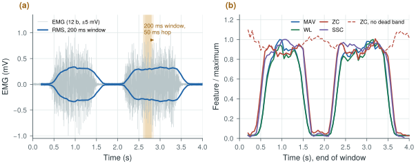
biosig.emg() with 3.4 µVrms of noise, quantised to 12 bits over ±5 mV, and the RMS envelope over 200 ms windows that advance by 50 ms (one window and its successor shaded). (b) MAV, WL, ZC and SSC per window, each divided by its maximum; ZC and SSC use a 20 µV dead band. Without it (dashed) ZC counts noise at rest and reads higher there than in the contraction. Computed in figsrc/ch26_figs.py.Frequency-domain features (median and mean frequency of the spectrum) track muscle fatigue, which shifts the spectrum downwards during a sustained contraction.
26.2Gesture classification
Each hand gesture activates a different combination of forearm muscles, so the pattern of features across several electrode channels identifies the gesture. A linear discriminant on MAV, WL, ZC and SSC from eight channels is the classic baseline, and the NinaPro database [6] the standard benchmark.
figsrc/ch26_figs.py generates synthetic 8-channel EMG for five gestures, each a fixed pattern of channel amplitudes (0.03–0.6 mVrms) with trial-to-trial variation of ±25 % per channel and ±30 % overall, plus 3 µVrms of noise. It computes the four features per channel over 200 ms and trains a linear discriminant on 40 trials per gesture (Figure 26.2). Over the EMG-mode range of ±5 mV:
- with 5 bits or more, accuracy is 100 % at 500, 1000 and 2000 S/s;
- with 4 bits, 98–99.5 %; with 3 bits, 57–66 %, against 20 % chance.
The synthetic gestures are well separated by construction. Real recordings, with dozens of gestures, electrode shift and fatigue, are much harder, and NinaPro results depend more on the number of channels, the electrode placement and the training data than on the converter. The design point stands: gesture recognition uses only a handful of bits, and sample rates well below 2 kS/s.
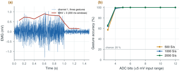
figsrc/ch26_figs.py.26.3Windows, latency and the feature engine
A prosthesis needs a stream of decisions, not one per gesture. The features are therefore computed over a window \(W\) that slides forward by a hop \(H\), overlapping its predecessor when \(H < W\): a dense decision stream from long, low-noise windows, the usual scheme in myoelectric control [65]. Two numbers follow. The latency: after a step in muscle activity a window is half full of the new activity after \(W/2\), and the next decision comes up to \(H\) later, so the features reach half their new value after \(W/2 + H/2\) on average and \(W/2 + H\) at worst. The envelope noise of a window falls as \(1/\sqrt{W}\).
At 2 kS/s, a 200 ms window holds 400 samples and a 50 ms hop adds 100 new ones.
- Decisions: \(1/H\) = 20 per second, each from 8 channels × 4 features = 32 numbers: 640 features per second.
- Latency to half the change: 125 ms on average and 150 ms at worst. Moving the onset of a
biosig.emg()contraction across one hop gives 127 and 167 ms; the simulated onset is a smooth rise (10–90 % in about 180 ms), and the estimate fluctuates. - Without overlap (\(H = W\)): 5 decisions per second, 200 ms on average and 300 ms at worst (simulated 198 and 300 ms).
- Envelope noise: in a steady contraction the MAV of a 200 ms window varies by 5.5 % rms; 100 ms gives 7.7 %, 50 ms 11.0 %, 25 ms 15.5 %.
A 100 ms window with a 25 ms hop halves the delay (65 ms simulated) for 1.4 times the noise and 40 decisions per second. 200 ms with a 50 ms hop is a sound default: 5.5 % is small next to the ±25 % trial-to-trial variation of Worked Example 26.1, and the delay is about an eighth of a second.
With block sums the overlap is free: MAV, WL, ZC and SSC are sums, so the chip accumulates them over 50 ms blocks and adds the last four for each 200 ms window.
For each channel and each new sample, feature_engine() in figsrc/ch26_figs.py does:
- the magnitude \(\lvert x[n]\rvert\) and its accumulation: 2 operations (for the SAR’s mid-rise codes the magnitude of a negative code is its bitwise complement);
- the step \(d[n]\), its magnitude and its accumulation into WL: 3;
- the dead-band compare \(\lvert d[n]\rvert \ge T\), shared by ZC and SSC: 1;
- ZC: compare the sign bits of \(x[n]\) and \(x[n-1]\), and count: 2;
- SSC: compare the sign bits of \(d[n]\) and \(d[n-1]\), combine with the two dead-band flags, and count: 3.
That is 11 additions, compares or bit operations and no multiplication per sample: 22 000 per second per channel, 176 000 for eight. Adding four block sums per feature every 50 ms adds about 1 %. At an assumed 1 pJ per operation, an order-of-magnitude figure for 16-bit logic in 130 nm, the engine draws about 0.2 µW.
Word lengths. With 8-bit inputs, the sum of 400 magnitudes stays below 400 × 128 = 51 200 (16 bits), WL below 400 × 255 (17 bits), ZC and SSC below 400 (9 bits); with all 12 bits, 20 and 21 bits. The integer engine matches the floating-point MAV exactly and ZC and SSC to within one count.
Data. Raw EMG, 8 × 2 kS/s × 12 b, is 192 kb/s. Features as 16-bit words are 2.56 kb/s at 5 windows per second, 75 times less (the budget of Chapter 27), and 10.2 kb/s at 20 per second, 19 times less. If the linear discriminant also runs on chip (160 multiply–accumulates per decision: 5 classes × 32 features), only a 3-bit class label leaves: 60 b/s, 3 200 times less. At Chapter 27’s order-of-magnitude 5 nJ per radio bit, that is 960 µW for raw data against 13, 51 or 0.3 µW.
Build the EMG feature engine from block accumulators: no multiplier (MAV, not RMS), 16-bit sums from 8-bit inputs, and a programmable dead band a little above the noise. Choose the window for envelope noise and the hop for latency. The engine costs a fraction of a microwatt and saves most of a milliwatt of radio, so it belongs on the chip, and the classifier can follow it: Lab 13 keeps 100 % accuracy with 6-bit weights.
26.4Spike detection
An extracellular spike is 50–500 µV tall and about a millisecond long, riding on background noise and on slower local field potentials (Chapter 2). A simple amplitude threshold, typically four to five times the noise’s standard deviation, works when the spikes are large. The standard deviation must be estimated robustly, from the median absolute value, because spikes inflate a plain standard deviation but barely move the median [68]:
For Gaussian noise the median of \(\lvert x\rvert\) is \(0.6745\sigma\), the 75th percentile of the normal distribution. \(Q(k)\) is the probability that one noise sample lies beyond \(k\sigma\): \(3.2\times10^{-5}\) at 4σ, \(3.4\times10^{-6}\) at 4.5σ, \(2.9\times10^{-7}\) at 5σ. Excursions that far last 20–24 µs on average for this noise, less than a sample period at 20–30 kS/s, so each is caught by about one sample and \(R_\mathrm{FA} \approx f_\mathrm{s}Q(k)\). (An analog comparator sees them all: Rice’s level-crossing rate \(\nu_0 e^{-k^2/2}\), with \(\nu_0 \approx 3.9\) kHz the rms frequency of the noise, gives 1.3 per second at 4σ.)
Take biosig.spikes() at 30 kS/s, with 8 µVrms of background noise and spikes of 105–150 µV, 1 182 of them in 60 s (19.7 per second).
- Noise estimate. The plain standard deviation is 12.0 µV, 50 % high, because it counts the spikes as noise; the median estimate gives 8.19 µV, 2 % high.
- Threshold. At \(k\) = 4.5 it is −36.9 µV from the median but −54.0 µV from the standard deviation, which would miss most spikes smaller than that.
- False alarms on noise alone, over 1 200 s: 0.88 per second at 4σ, 0.11 at 4.5σ and 0.012 at 5σ, against \(f_\mathrm{s}Q(k)\) = 0.95, 0.10 and 0.009. At 20 kS/s: 0.65, 0.068 and 0.004 per second.
- Spikes. A 4.5σ threshold adds one false event for every 180 true ones. Every spike crosses even 5σ; the 19 missed (1.6 %) arrive within 1 ms of another spike, inside the 1 ms dead time.
For large spikes \(k\) hardly matters. For small ones it does: with troughs of 35–50 µV (4.3–6.1σ) the detector finds 95.9 % at 4σ, 89.7 % at 4.5σ and 77.3 % at 5σ (Figure 26.3b). Choose \(k\) from the false-alarm rate that spike sorting downstream can tolerate.
The nonlinear energy operator (NEO) [66] is the classic alternative to a fixed threshold, and it can work better for small, sharp spikes:
\(\psi\) is large where the signal is both large and changing quickly, so it emphasises spikes over slower, equally large background fluctuations. A threshold on a smoothed \(\psi\), at a multiple of its mean, detects the spikes. It costs two multiplications per sample, which suits an implant.
How much it helps depends on what is slower than the spike. A 100 µV local field potential at 10 Hz gives \(\psi = A^2\sin^2(2\pi f/f_\mathrm{s}) = 4.4\times10^{-14}\) V² at 30 kS/s, nearly five thousand times less than the \(2.1\times10^{-10}\) V² of a 50 µV spike, so the NEO ignores the LFP and drift that defeat a fixed threshold. In Open-BioAFE’s spike mode, however, the 300 Hz high-pass has already removed the LFP, and the remaining noise fills the band to 7 kHz: it is faster than the spike. At 30 kS/s a spike’s trough spans several samples, so \(x[n-1]\,x[n+1] \approx x[n]^2\) and the peak \(\psi\) of a 50 µV spike is only \(3.2\sigma^2\), against a noise mean of \(0.87\sigma^2\). Stretching the operator to the spike’s time scale, \(\psi_\ell[n] = x[n]^2 - x[n-\ell]\,x[n+\ell]\) with a lag \(\ell\) = 5 samples (0.17 ms) [67], raises the peak to \(35.8\sigma^2\) against \(1.05\sigma^2\).
On the small spikes over 400 s (Figure 26.3), at one false alarm per second the plain NEO smoothed over five samples finds 10 % (26 % unsmoothed), the amplitude threshold 96.4 % and the lag-5 NEO 97.6 %; at 0.1 per second, 3.4, 91.3 and 96.0 %. The NEO is also blind to polarity, so it finds positive-going spikes that a one-sided threshold misses.
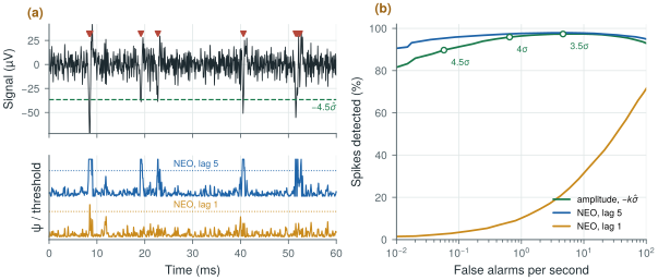
biosig.spikes() at 30 kS/s with 8 µVrms of noise and spikes of 35–50 µV (triangles), with the threshold at \(-4.5\hat\sigma\). Bottom: the NEO at lag 1 and lag 5, smoothed over five samples and divided by the threshold that gives one false alarm per second (dotted). (b) Spikes detected against false alarms per second as the threshold is swept, over 400 s; the open circles mark the amplitude threshold at 3.5σ, 4σ and 4.5σ. At lag 1 the NEO responds to the noise as much as to the spikes. Computed in figsrc/ch26_figs.py.On chip, the median needs no stored record. The running estimate \(m \leftarrow m + \delta\,\mathrm{sign}(\lvert x[n]\rvert - m)\) settles where \(\lvert x\rvert\) exceeds \(m\) half the time, which is the median, for one compare and one addition per sample. With 12-bit codes over the spike mode’s ±0.625 mV (±0.5 V over the gain of 800 in Table 11.1) and \(\delta = 2^{-8}\) LSB, it settles to within 5 % in 0.5 s and then wanders by 2 % rms.
In the 300 Hz–7 kHz band of spike mode, a negative threshold at \(4\ldots4.5\,\hat\sigma\), with \(\hat\sigma\) from a running median, costs two compares and an addition per sample and loses only a few percent to the best detector here. Set \(k\) from the false alarms you can afford: about one per second at 4σ, one per ten seconds at 4.5σ. Offer the NEO with a programmable lag (about 5 samples at 30 kS/s, 3–5 at 20 kS/s) for spikes of either polarity or a band that reaches into the LFP; at lag 1 on an oversampled spike it is the wrong tool.
26.5Spike sorting and compression
Each electrode records several neurons, whose spikes differ in shape. Spike sorting extracts each detected spike’s waveform, reduces it to a few features (principal components or wavelet coefficients), and clusters them, one cluster per neuron. The full process is computationally heavy and is normally done off the implant.
Implants compress because their radio, not their front-end, limits them. Ten channels at 30 kS/s and 10 bits are 3 Mb/s of raw data, more than an implantable link can sustain within its heat budget. Sending only the spike times (a few bytes per spike, at tens of spikes per second per channel) reduces that by two to three orders of magnitude. Sending short waveform snippets around each spike, so that sorting can be done outside, sits in between. Chapter 27 budgets the radio.
One channel at 30 kS/s and 12 bits is 360 kb/s. The recording of Worked Example 26.4 carries 19.7 spikes per second, one event for about every 1 500 samples. The chip can send:
- spike times only, as 32-bit sample counts: 0.63 kb/s, 570 times less;
- times and 16 twelve-bit samples per spike, the budget of Chapter 27 at 30 spikes per second: 6.7 kb/s, 54 times less;
- times and the full 1.6 ms snippet, 48 samples at 30 kS/s, at 8 bits: 8.2 kb/s at 19.7 spikes per second and 12.5 kb/s at 30, 44 and 29 times less.
Eight bits suffice for the snippet: over ±0.625 mV one LSB is 4.9 µV and its quantisation noise 1.4 µVrms, under a third of the 8 µVrms background, the rule of Chapter 13. Ten channels, 3 Mb/s raw at 10 bits, need 82–125 kb/s with snippets and 6–10 kb/s with times alone.
For EMG, compute the time-domain features on chip over 100–250 ms windows; they need few bits and modest sample rates, and cut the data 19 to 75 times, or 3 200 times as class labels. More channels and good electrode placement improve gesture recognition far more than more bits. For spikes, detect on chip with an amplitude threshold from a running median, or a NEO with its lag matched to the spike, and send spike times or short snippets, never the raw 30 kS/s stream.
EMG mode: MAV, WL, ZC and SSC per channel over 200 ms windows every 50 ms from the 2 kS/s, 12-bit SAR data (features computed on 8-bit inputs, 16-bit block accumulators, programmable dead band), streamed at 5–20 windows per second (2.6–10 kb/s), or class labels when the classifier runs on chip. Spike mode (one channel, optional): threshold at \(-k\hat\sigma\) (\(k\) programmable, default 4.5) from a running median, NEO with programmable lag as an option, 1 ms dead time; spike times and 1.6 ms snippets (48 samples, 8 bits).
Testing a gesture classifier on trials recorded in the same session as its training data. Electrode position, skin condition and fatigue change from session to session, and accuracy measured within a session overstates what a user will see. Train and test on different sessions, or different days, and report both.
Lab 13 computes MAV, WL, ZC and SSC on NinaPro, trains LDA or SVM classifiers in fixed point, and plots accuracy against channels, sample rate and resolution. Run figsrc/ch26_figs.py first, then replace its synthetic windows with NinaPro recordings; if NinaPro needs registration, provide a local file or keep the synthetic fallback. For spikes, vary the amplitude, lag and smoothing in its detectors (sigma_hat(), neo(), detect()) and compare with Figure 26.3b.
Read with this chapter. The NinaPro database [6], Buzsáki, Anastassiou and Koch [36] (extracellular signals and spikes). Hudgins, Parker and Scott [64] and Englehart and Hudgins [65] for the EMG features and overlapped windows; Mukhopadhyay and Ray [66], Choi, Jung and Kim [67] and Quian Quiroga, Nadasdy and Ben-Shaul [68] for the NEO, its multi-resolution form and the median threshold.
- EMG is read through its envelope: MAV, WL, ZC and SSC over 100–250 ms windows; ZC and SSC need a dead band, or noise at rest reads as frequency.
- In a synthetic five-gesture study a linear discriminant reaches 100 % with 5 bits over ±5 mV at 500–2000 S/s; real recordings depend more on channels and placement than on bits.
- A 200 ms window every 50 ms gives 20 decisions per second, about 125 ms of delay and 5.5 % envelope noise. The engine needs 11 additions or compares per sample, about 0.2 µW for eight channels, and cuts 192 kb/s to 2.6–10 kb/s, or 60 b/s of class labels.
- Estimate spike noise as \(\operatorname{median}\lvert x\rvert/0.6745\), not the standard deviation; a threshold at \(k\hat\sigma\) gives about \(f_\mathrm{s}Q(k)\) false alarms per second, 0.9 at 4σ and 0.1 at 4.5σ at 30 kS/s.
- The nonlinear energy operator \(x[n]^2 - x[n-1]x[n+1]\) costs two multiplications per sample, but at 30 kS/s it needs a lag of about five samples to match an amplitude threshold; its strength is ignoring slow LFP and drift.
- Implants send spike times or snippets, not raw data: 360 kb/s per channel becomes 0.6–12.5 kb/s. The radio, not the front-end, sets the limit.