Chapter 33Closed-Loop Systems
A device that only records can be slow; a device that acts on what it records must decide in time, and timing becomes part of the specification.
- describe closed-loop biomedical systems: sense, decide, act;
- build a latency budget from the electrodes to the stimulus, and turn it into a phase error;
- estimate the phase of a brain rhythm in real time, despite the delay of every causal filter;
- time stimuli to samples, and keep stimulus artefacts out of the recording;
- measure evoked responses by averaging, and size the recording for them.
Where must the loop close, on the device or beyond the radio, for the stimulus to land at the right moment of the rhythm it targets?
Up to now the chip has listened. A closed-loop system also acts: it detects a state in the signal and responds within a fixed time, by stimulating a nerve, playing a sound, vibrating, or changing a therapy. Responsive neurostimulators detect the onset of a seizure and stimulate to stop it (Chapter 27). Sleep studies play short bursts of sound timed to the slow oscillations of deep sleep and enhance them [59]. Brain-stimulation studies time each pulse to the phase of an ongoing rhythm, because the brain’s response depends on it [60]. Hearing tests at the ear play sounds and measure the brain’s response to them. All share one requirement that open-loop recording never had: a deadline.
33.1Sense, decide, act
A closed loop has four stages: acquisition (electrodes, front-end, converter and decimation), decision (filtering, detection, phase estimation), actuation (a sound, a current, a vibration) and the body’s own response. Each stage adds delay, and the decision stage must work only with the past: every filter it uses is causal, and every causal filter delays the signal.
33.2The latency budget
Add up the delay from the electrodes to the stimulus:
- Conversion. An incremental ΔΣ conversion takes its whole cycle: 2 ms at 500 S/s (Chapter 20). A SAR samples in microseconds.
- Digital filters. A linear-phase FIR filter of \(N\) taps delays every frequency by \((N-1)/2\) samples; a band-pass that isolates a 1 Hz rhythm needs a long filter, and so a long delay.
- The link. Over BLE, a sample waits in a buffer for the next connection event, then for the phone’s scheduler: tens of milliseconds, with a jitter of the same order (Chapter 27).
- The actuator. An audio codec’s output buffer, a stimulator’s ramp-up: a few milliseconds.
A latency \(\tau\) that is not compensated becomes a phase error \(\Delta\varphi\) at the rhythm’s frequency \(f\); a jitter in \(\tau\) becomes a phase jitter by the same rule.
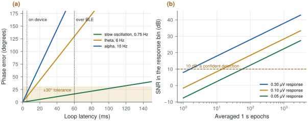
Figure 33.1a draws the rule for three rhythms. For the slow oscillation of deep sleep, about 0.75 Hz, a 60 ms loop over BLE costs 16°, inside a ±30° tolerance. For theta at 6 Hz it costs 130°, and for alpha at 10 Hz 216°: the stimulus lands on the opposite phase. A loop that closes on the device, within about 5 ms, keeps alpha within 18°. Fast rhythms need the loop on the device; slow ones can tolerate the radio, if its jitter is controlled.
figsrc/ch33_figs.py.33.3Estimating the phase in real time
The textbook way to find the phase of a rhythm, a zero-phase band-pass filter and the Hilbert transform, needs the future: it filters forwards and backwards. A real-time system has only the past. Three practical approaches:
- Filter and predict. Band-pass the recent signal causally, fit a short autoregressive model to it, and forecast the next fraction of a second; take the phase from the forecast at the present moment. This compensates the filter’s delay and is the approach behind phase-locked brain stimulation [60].
- Track the rhythm with a phase-locked loop: an oscillator whose phase is pulled towards the band-passed signal, updated every sample, cheap enough for a small datapath.
- Detect events and extrapolate: for the slow oscillation, detect the negative half-wave when it crosses a threshold and schedule the sound for the expected up-phase a fixed time later [59].
All three degrade when the rhythm is weak or irregular. A good loop measures its own accuracy, by logging the true phase afterwards with a zero-phase filter, and acts only when the rhythm is present and the signal-quality index of Chapter 31 says the data can be trusted.
The demo below runs the simplest real-time scheme, event detection: a causal band-pass at the target frequency, an upward zero crossing as the event, and a stimulus aimed at the next peak a quarter period later, delivered after the loop’s latency and jitter. The true phase of each stimulus is found afterwards with a zero-phase filter and the Hilbert transform. It starts at a 0.75 Hz slow oscillation and 60 ms through a radio link; move the frequency to alpha.
33.4Acting without corrupting the recording
The stimulus must be timed by the same clock as the samples. An audio codec clocked from the front-end’s reference (Chapter 29) plays its sounds on known samples, so every stimulus can be placed exactly in the recording; a codec on its own crystal drifts against the EEG by a sample every few tens of seconds.
The stimulus must also stay out of the recording, or the loop responds to its own output. Electrical stimulation couples directly into the electrodes (Chapter 27): the front-end must survive it without saturating, and the samples during each pulse are blanked or flagged. Sound reaches the EEG through the speaker’s magnetic field, the drive currents and the mechanics of the earpiece: separate grounds, a speaker driver away from the inputs, and stimulus timing logged with the data keep it identifiable.
33.5Evoked responses: hearing tests at the ear
A closed loop can also test. Play a sound and measure the brain’s response: an auditory brainstem response (ABR) to clicks, a few milliseconds long, or an auditory steady-state response (ASSR) to a tone modulated at, typically, 40 or 80–100 Hz [61]. Both are far smaller than the background EEG, so they are measured by averaging: the response repeats with every stimulus while the EEG does not, and the noise falls as \(1/\sqrt{N}\) over \(N\) repetitions. An ASSR appears as a peak at its modulation frequency in the averaged spectrum, detected when it stands far enough above the neighbouring bins. At the ear the responses are smaller still [57]: Figure 33.1b shows that a 0.1 µV response needs about 15 averaged seconds at the noise of a dry ear-EEG channel, and a 0.05 µV one about a minute.
The requirements differ from those of continuous EEG. An ASSR at 80–100 Hz needs bandwidth well above the sleep and alpha bands; an ABR needs tens of kilosamples per second and stimulus timing accurate to tens of microseconds. For Open-BioAFE, that is the 16 kS/s SAR path of Chapter 18, not the 500 S/s ΔΣ path, with the stimulus clocked from the same reference as the converter.
Write the latency budget before the architecture: if the target rhythm is fast, the decision must run on the device, next to the converter. Clock the stimulus from the converter’s reference, log every stimulus with the samples, blank or flag the samples it corrupts, and act only when the signal-quality index allows. For evoked responses, budget the averaging time from the input noise, and give the converter the bandwidth and the timing accuracy the response needs.
Quoting a closed loop’s mean latency and forgetting its jitter. A loop through a phone that averages 40 ms but varies by ±20 ms spreads its stimuli over ±72° of a 10 Hz rhythm, even if the mean has been compensated. Measure the latency distribution end to end, from a test signal at the electrodes to the stimulus at the actuator.
Generate a slow oscillation with biosig.eeg() plus a 0.75 Hz component, band-pass it causally, and schedule a “sound” a fixed delay after each negative half-wave crosses −40 µV. Measure the true phase of each stimulus afterwards with a zero-phase filter and the Hilbert transform, and plot its spread against the noise level and the delay. Then change the numbers in figsrc/ch33_figs.py to your own noise and response amplitude.
Read with this chapter. Ngo et al. [59], Zrenner et al. [60], Picton et al. [61], Kidmose et al. [57].
- A closed loop senses, decides and acts within a deadline; every causal filter and every buffer in it adds delay.
- A latency τ is a phase error 360°·f·τ: 60 ms over BLE costs 16° of a 0.75 Hz slow oscillation but 216° of 10 Hz alpha.
- Real-time phase needs prediction (an autoregressive forecast), a phase-locked loop or event detection, and a check of its own accuracy.
- Clock the stimulus from the converter’s reference, log it with the samples, and keep its artefacts out of the decision.
- Evoked responses are averaged: noise falls as 1/√N; at dry ear-EEG noise a 0.1 µV ASSR needs about 15 s. ABRs need the fast SAR path and microsecond timing.