Chapter 27On-Chip Processing and System Integration
On a wearable or implant, the radio usually costs more energy than the sensing; computing on chip is how you spend less of it.
- place feature extraction and small machine-learning models in silicon;
- use the seizure-detection SoC of Verma et al. [25] as a case study;
- compress biosignal data before transmission;
- design power management with LDOs and energy harvesting;
- compare BLE, backscatter and inductive data links;
- size a BLE link for raw and feature streams: PHY, connection interval, payload, buffer and radio power;
- introduce stimulation: current DACs and charge balance.
Which processing belongs on the Open-BioAFE chip, and which data must leave it?
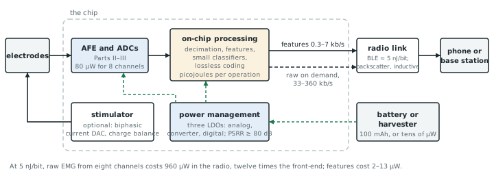
Chapters 24–26 found that heartbeats, seizures and gestures can be recognised from a few numbers per window. This chapter asks what that is worth in a system, where the front-end is only one consumer among several, and adds the remaining pieces of a complete biosignal chip: power management, the data link and, briefly, stimulation (Figure 27.1).
27.1Feature extraction and edge ML in silicon
Every bit that leaves the chip costs energy in the radio; every operation on chip costs energy in the logic. The comparison decides the partition.
Eight channels of raw samples need 64 kb/s for ECG (500 S/s, 16 bits), 33 kb/s for EEG (256 S/s, 16 bits) and 192 kb/s for EMG (2 kS/s, 12 bits); one spike channel at 30 kS/s and 12 bits needs 360 kb/s. The features of the previous chapters need 0.3 kb/s (RR intervals and rhythm flags), 0.4 kb/s (six band powers per 2 s window and channel), 2.6 kb/s (four features per channel at five windows per second) and 6.7 kb/s (spike times and 16-sample snippets): 54 to 190 times less (Figure 27.2a).
A Bluetooth-Low-Energy-class radio costs of the order of 5 nJ per transmitted bit, all overheads included. Raw EMG then costs 960 µW in the radio, twelve times the 80 µW of the whole eight-channel front-end; raw ECG 320 µW; the features 2–13 µW (Figure 27.2b).
The features cost little to compute. Band power is a filter, a squarer and an accumulator per band; MAV, WL, ZC and SSC are additions and comparisons; Pan–Tompkins is a few filters and a threshold. In a 130 nm process these operations cost picojoules each, and the feature path runs on the decimated, reduced-word-length data of Part IV. Small classifiers, such as a linear discriminant, a decision tree or a support-vector machine with a handful of support vectors, fit as well, especially with per-patient training done offline and only the parameters loaded on chip.
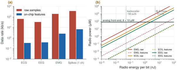
figsrc/ch27_figs.py; the energy-per-bit values are order-of-magnitude assumptions.27.2Case study: an EEG seizure-detection SoC
The SoC of Verma et al. [25] is the reference design for this partition: chopper-stabilised instrumentation amplifiers, a multiplexed SAR converter and a feature processor that computes spectral energy features on chip, so that a seizure detector can run on the features rather than on raw EEG streamed off the device. Reading it after Part IV, look for three numbers: the energy of the analog front-end per channel, the energy of the feature computation per channel, and the data rate the chip would need without the features. The pattern of this chapter, in which features cost far less than transmission, is what made the design worthwhile.
27.3Compression
When raw data must leave the chip, for clinical review or for training a classifier, compression reduces the cost. Lossless coding of the differences between successive samples, with a variable-length code such as a Huffman or Rice code, typically halves to thirds the data for ECG and EEG, because successive samples are close. Lossy methods, such as transform coding with wavelets, level-crossing sampling (Chapter 21) or compressive sensing, go further at a controlled loss of fidelity. Spikes are compressed by detection itself, as Chapter 26 showed. Lossless difference coding is cheap enough for any chip and should be the default for raw streams.
27.4Power management
A microvolt front-end needs a quiet supply. A low-dropout regulator (LDO) between the battery and the analog circuits suppresses the battery’s and the digital circuits’ noise, but adds its own: an LDO’s output noise of a few tens of microvolts across the band is common, and it reaches the signal through the front-end’s limited power-supply rejection. With 80 dB of PSRR, 30 µVrms becomes 3 nVrms at the input, which is harmless; with 40 dB it becomes 0.3 µVrms, a fifth of the EEG budget. Separate LDOs for the analog front-end, the converters and the digital logic, and a fully differential front-end, keep the PSRR high. Clock edges and digital switching currents must stay off the analog supply and substrate.
Wearables run from small batteries, typically tens to hundreds of milliampere-hours. At 1.2 V and 100 µW for the whole chip, a 100 mAh cell lasts about 50 days. Energy harvesting (thermoelectric from body heat, photovoltaic, or radio-frequency power) delivers tens of microwatts at best on the body, which a feature-transmitting chip can live on and a raw-streaming one cannot.
27.5Data links
Three kinds of link dominate:
- Active radios such as BLE: standard, interoperable with phones, of the order of nanojoules per bit, and duty-cycled to save power at low data rates.
- Backscatter: the chip modulates the reflection of a carrier sent by a reader, instead of generating its own; tens to hundreds of picojoules per bit on the chip side, but the reader must be close and powered.
- Inductive links for implants: a coil pair carries both power and data through the skin, with data rates from tens of kilobits to megabits per second.
The link chooses itself once the data rate is known: features fit any of them; raw spikes or raw multichannel EMG need a capable, power-hungry link or a wire.
27.6Getting the data out over BLE
Bluetooth Low Energy is the link almost every wearable uses, because every phone already speaks it [49, 50]. Its cost per bit is only half the story; the other half is how a continuous stream fits a protocol built for short, infrequent messages.
How a BLE connection moves data. The phone (the central) and the sensor (the peripheral) meet at connection events, one every connection interval \(T_\mathrm{CI}\), from 7.5 ms to 4 s, chosen by the central. In each event the peripheral sends some number of packets, each acknowledged before the next, and both radios then sleep until the next event. Each packet carries one link-layer payload: 27 bytes in the original specification, up to 251 bytes with Data Length Extension. After the L2CAP and ATT headers (7 bytes), an ATT notification carries 20 or 244 bytes of your data. The radio runs at 1 Mb/s (LE 1M PHY) or, since Bluetooth 5, at 2 Mb/s (LE 2M); the Coded PHY trades rate (500 or 125 kb/s) for range.
\(L\) is the ATT payload (20 or 244 bytes), \(N_\mathrm{pkt}\) the packets per event, \(t_\mathrm{IFS}\) = 150 µs the gap between packets. In practice the phone also caps \(N_\mathrm{pkt}\), often at four to seven, and sets a minimum interval, often 15 ms.
A 244-byte notification on an encrypted link is 265 bytes on air with preamble, access address, header, MIC and CRC: 2.12 ms at 1 Mb/s. With the two 150 µs gaps and the central’s 80 µs empty acknowledgement, one packet takes 2.50 ms, so the link tops out at \(244 \times 8 / 2.50\ \text{ms} \approx\) 780 kb/s. At 2 Mb/s the same packet takes 1.41 ms: about 1.4 Mb/s. Those are ceilings. With the original 20-byte payload and a phone that allows four packets every 30 ms, the same radio carries \(4 \times 20 \times 8 / 30\ \text{ms} =\) 21 kb/s.
Fitting Open-BioAFE’s streams. Add about 4 % for framing (below) to the raw rates of section 27.1:
| Stream | Rate | A BLE setting that carries it |
|---|---|---|
| features, any mode | 0.3–7 kb/s | 1M PHY, 20-byte payload, interval 100–500 ms |
| raw EEG, 8 × 256 S/s × 16 b | 34 kb/s | 1M, 244-byte payload, 50 ms, 1–2 packets per event |
| raw ECG, 8 × 500 S/s × 16 b | 67 kb/s | 1M, 244-byte payload, 30 ms, 2 packets |
| raw EMG, 8 × 2 kS/s × 12 b | 200 kb/s | 2M, 244-byte payload, 15 ms, 2 packets |
| one spike channel, 30 kS/s × 12 b | 375 kb/s | 2M, 244-byte payload, 15 ms, 3 packets |
| ten spike channels | 3.7 Mb/s | does not fit: send spike times or snippets (Chapter 26) |
What it costs. A useful first model of the radio’s average power is \(P \approx E_b R + E_\mathrm{ev}/T_\mathrm{CI}\): an energy per bit \(E_b\) of a few nanojoules (about 5 nJ at 1M, nearer 3 nJ at 2M, where each bit spends half as long on air) plus a fixed cost \(E_\mathrm{ev}\) for every event, of the order of 10 µJ for waking the radio, starting its crystal and exchanging the empty packets. Both numbers are order-of-magnitude assumptions; read your radio’s power profiler for real ones. Raw ECG at a 30 ms interval then costs about 0.34 mW for the bits and 0.33 mW for the events. Stretch the interval to 100 ms, sending more packets per event, and the total falls to about 0.44 mW; send features at 500 ms and it is about 30 µW, close to the front-end’s own power. Long intervals and full packets are the cheapest way to move the same bits.
Buffering. Between events the samples wait in a FIFO, in the front-end or in the radio’s processor. It must hold at least \(R\,T_\mathrm{CI}\), and in practice three to five times that, because the link layer retransmits a lost packet at the next event and the phone sometimes skips events: raw EMG at 15 ms needs about 1.5 kB.
Framing, loss and time. Open-BioAFE’s SPI port and its data-ready line (the specification at the end of this chapter) feed a BLE system-on-chip, which reads each frame and packs whole frames into notifications. Give every notification a small header: a sequence number, so that a gap shows a lost packet, and the converter’s sample counter, so that the receiver places the samples in time by the chip’s own clock, not by when the packet arrived. For raw ECG, an 8-byte header and 14 frames of 8 channels × 16 bits make a 232-byte notification, 3.4 % of overhead. BLE’s link layer already retransmits until each packet is acknowledged, so data is lost only when the connection drops or a FIFO overflows; the sequence numbers make either visible.
Two devices, one time base. Two sensors, one on each ear or one on each arm, have independent clocks. Even 50 ppm apart, two 500 S/s streams slip by one sample every 40 seconds. Timestamps by sample counter, realigned at regular sync points, fix that in software; Bluetooth 5.2’s isochronous channels, built for LE Audio, give both devices common anchor points; and two devices wired together can simply share one clock.
27.7Stimulation
Closed-loop devices, such as responsive neurostimulators and functional electrical stimulation, also deliver current through electrodes. A stimulator is a current-steering DAC that drives biphasic pulses: a cathodic phase that excites the tissue and an anodic phase that returns the charge. Charge balance is the safety requirement: any net charge left on the electrode drives electrochemical reactions that corrode the electrode and damage tissue. Matched current sources, passive shorting of the electrodes between pulses, and series DC-blocking capacitors keep the residual charge near zero. The recording front-end must also survive the stimulation artefact, volts at the electrode for milliseconds, which is where the large input range of direct-digitising front-ends (Chapter 21) and the fast recovery of the servo loop (Chapter 10) matter. Sarpeshkar [12] treats both the energy-efficient electronics and the systems around them.
Compute the features on chip and send them, with raw data only on demand and losslessly compressed: at nanojoules per radio bit, raw multichannel data costs ten times the front-end, features a small fraction of it. Give the analog front-end its own quiet LDO and keep its PSRR high. Choose the link from the data rate, not the other way round. If the device stimulates, design charge balance in from the start.
On chip: decimation, the feature paths of Chapters 24–26 (RR intervals, band powers, EMG features, spike times) and lossless difference coding for raw streams. Out: an SPI interface to an external BLE or backscatter radio, features by default (0.3–7 kb/s), raw data on demand. Separate analog, converter and digital LDOs; front-end PSRR ≥ 80 dB. No stimulator in the first revision.
Quoting a microwatt front-end and leaving out the radio. A wearable’s battery life is set by the whole system, and with raw streaming the radio usually dominates by an order of magnitude. Budget the link with the front-end from the first page (Chapter 29).
Add a lossless Rice coder to figsrc/ch27_figs.py and measure its compression ratio on biosig.ecg() and biosig.eeg() samples quantised to 16 bits; then recompute the raw-data radio power with the compressed rate.
Read with this chapter. Verma et al. [25], Sarpeshkar [12] (ultra-low-power bioelectronics).
- On-chip features cut the data by 54 to 190 times (ECG, EEG, EMG, spikes).
- At about 5 nJ per radio bit, raw EMG from eight channels costs 960 µW, twelve times the front-end; features cost 2–13 µW.
- Lossless difference coding halves to thirds raw ECG and EEG; spikes are compressed by detection.
- The front-end needs its own LDO and high PSRR: 80 dB turns 30 µV of supply noise into 3 nV.
- Links: BLE (nanojoules per bit), backscatter (tens of picojoules), inductive for implants; the data rate chooses.
- BLE carries about 780 kb/s at 1M and 1.4 Mb/s at 2M at best, tens of kb/s on default settings; raw ECG, EEG and EMG fit with long payloads, many-channel spikes do not. Long intervals and full packets save power; timestamp every packet with the sample counter.
- Stimulators must be charge-balanced; the recording front-end must survive their artefacts.