Chapter 19ΔΣ Modulation: Theory
Oversample, quantise coarsely and push the quantisation noise out of the band: noise shaping turns a 1-bit quantiser into a 16-bit converter.
- derive the noise transfer function (NTF) and signal transfer function (STF) of first- and second-order loops;
- predict SQNR from loop order and oversampling ratio (OSR);
- check stability with the Lee criterion and understand idle tones and dither;
- synthesise an NTF and know how it maps to a loop topology;
- know when linearised analysis fails and simulation is needed.
Which loop order and OSR give 16 bits in the ECG/EEG band at the lowest clock rate?
Chapter 13 showed that plain oversampling buys only 3 dB per octave, and Chapter 14 that 16 bits at the Nyquist rate would need a 150 pF sampling capacitor. A ΔΣ modulator escapes both limits. It samples far faster than the signal needs, quantises with as little as one bit, and wraps the quantiser in a feedback loop that pushes the quantisation noise up in frequency, out of the narrow band where the biosignal lives. A digital filter then removes the out-of-band noise and lowers the rate. This chapter treats the loop as a mathematical object; Chapter 20 builds it.
The simulations in this chapter use biosig.simulate_dsm(), a 1-bit modulator written directly from its NTF. Every loop topology with the same NTF and an STF of one produces exactly the same output bits, so the results hold for whatever circuit Chapter 20 chooses. For real designs, Lab 9 uses python-deltasigma [27], the Python port of Schreier’s toolbox [10].
19.1Noise shaping
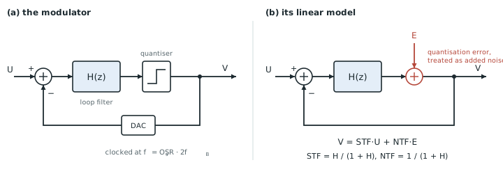
Put an integrator in front of a quantiser and feed the quantised output back, subtracting it from the input (Figure 19.1a). Model the quantiser as an adder that injects an error \(E\) (Figure 19.1b), as in Chapter 13, and let the integrator be \(z^{-1}/(1 - z^{-1})\). Then the output \(V\) obeys
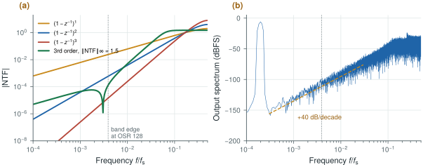
\[V = \frac{z^{-1}}{1 - z^{-1}}\,(U - V) + E \quad\Rightarrow\quad V = z^{-1}\,U + (1 - z^{-1})\,E.\]The input reaches the output delayed but otherwise untouched: the signal transfer function is \(\mathrm{STF}(z) = z^{-1}\). The quantisation error is filtered by the noise transfer function \(\mathrm{NTF}(z) = 1 - z^{-1}\), a differentiator. Its magnitude, \(\lvert\mathrm{NTF}\rvert = 2\sin(\pi f/f_\mathrm{s})\), is zero at DC, about \(2\pi f/f_\mathrm{s}\) in a narrow band, and 2 at \(f_\mathrm{s}/2\). The error power is unchanged, but it has been moved from low frequencies to high ones (Figure 19.2).
Two integrators in the loop give \(\mathrm{NTF} = (1 - z^{-1})^2\), three give the cube, and an order-\(L\) loop with a pure differentiator NTF shapes the noise as \(\lvert\mathrm{NTF}\rvert^2 \approx (2\pi f/f_\mathrm{s})^{2L}\) in band. Integrate the white error density \(\sigma_e^2/(f_\mathrm{s}/2)\) times this shape from 0 to the band edge \(f_\mathrm{B} = f_\mathrm{s}/(2\,\mathrm{OSR})\):
\[\sigma_\mathrm{in\text{-}band}^2 = \frac{2\sigma_e^2}{f_\mathrm{s}}\int_0^{f_\mathrm{B}} \left(\frac{2\pi f}{f_\mathrm{s}}\right)^{2L} df = \sigma_e^2\,\frac{\pi^{2L}}{(2L+1)\,\mathrm{OSR}^{2L+1}}.\]Compared with a full-scale sine, this gives the classical result:
biosig.ntf_response() and biosig.simulate_dsm().With a 1-bit quantiser (\(N = 1\), output levels ±1) and an OSR of 128, the formula gives, for a full-scale input,
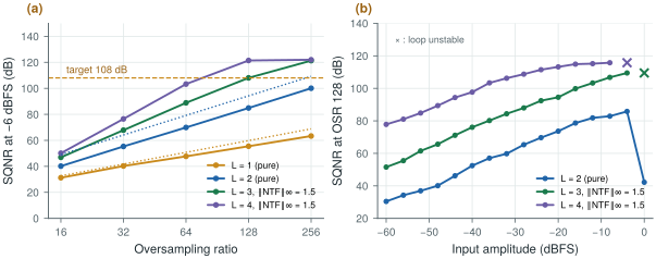
\[\mathrm{SQNR}_1 = 7.78 - 5.17 + 30\log_{10}128 = 65.8\ \text{dB}, \qquad \mathrm{SQNR}_2 = 7.78 - 12.9 + 50\log_{10}128 = 100.2\ \text{dB}.\]At a realistic −6 dBFS the predictions are 59.8 and 94.2 dB. The simulated modulators give 55.5 and 84.9 dB.
The second-order loop falls 9 dB short, and the reason is the 1-bit quantiser. The model assumes an error bounded by ±½ LSB with power \(\Delta^2/12 = 1/3\). In the loop, the quantiser’s input swings to about ±4, so its error is larger (the simulated error power is 0.55, 2 dB more), and the loop settles at an effective quantiser gain of about 0.63, which lifts the in-band shaped noise by another \(20\log_{10}(1/0.63) = 4\) dB. The error is also not white. The formula is a good guide to slopes and trends; the numbers you design with come from simulation.
19.2SQNR versus order and OSR
The formula’s most useful message is in its last term: every doubling of the OSR adds \((20L + 10)\log_{10}2 = 6L + 3\) dB. A first-order loop gains 9 dB per octave, a second-order one 15 dB and a third-order one 21 dB. Raising the order is far more effective than raising the clock, as long as the loop stays stable (section 19.3).
Table 19.1. Simulated SQNR (dB) of 1-bit modulators at −6 dBFS. Orders 1 and 2 use pure differentiators; orders 3 and 4 use NTFs synthesised for each OSR with \(\lVert\mathrm{NTF}\rVert_\infty = 1.5\) and optimised zeros. Values marked * are limited by the simulation’s record length, not by the loop.
| Order | OSR 16 | OSR 32 | OSR 64 | OSR 128 | OSR 256 |
|---|---|---|---|---|---|
| 1 | 31.3 | 40.3 | 47.7 | 55.5 | 63.3 |
| 2 | 40.2 | 55.3 | 69.9 | 84.9 | 100.1 |
| 3 | 46.9 | 67.8 | 88.9 | 108.1 | 121* |
| 4 | 50.1 | 76.5 | 103.3 | 121* | 122* |
Table 19.1 and Figure 19.3a show the slopes, and also the diminishing returns. The higher-order NTFs gain less per octave than \(6L + 3\) dB suggests, because their gain must be held down to keep the loop stable, which leaves more noise in band than a pure differentiator would. They also accept a smaller input before overloading. At low OSR the extra order buys little: at an OSR of 16 the four loops lie within 19 dB of each other.
To meet 16 bits, the converter’s total noise must sit 98 dB below full scale. If quantisation noise is to take no more than a tenth of that budget, leaving the rest for thermal noise, the modulator needs 108 dB at the largest input it will see. From the table: a third-order loop reaches it at an OSR of 128, a fourth-order one between 64 and 128, and a second-order one would need about 512.
biosig.simulate_dsm(), biosig.synth_ntf() and biosig.dsm_sqnr().The demo below runs a 1-bit modulator in your browser, 8192 cycles at a time, and reads its in-band SQNR the way biosig.dsm_sqnr() does. It starts at the second-order loop at OSR 128 and −6 dBFS of this section; change the order and the OSR, and compare the simulation with the linear model.
19.3Stability, idle tones and dither
A loop with a 1-bit quantiser is a nonlinear feedback system, and linear stability analysis does not cover it. The quantiser’s effective gain falls as its input grows, so a large input or a large internal state lowers the loop gain until the poles of the linearised loop leave the unit circle. The states then grow without bound: the loop is unstable, and the output is useless until the integrators are reset.
There is no exact test. The practical rule, the Lee criterion, says that a 1-bit loop is likely to be stable if its NTF never exceeds 1.5 in magnitude:
\[\lVert \mathrm{NTF} \rVert_\infty = \max_f \lvert\mathrm{NTF}(e^{j2\pi f/f_\mathrm{s}})\rvert < 1.5.\]A pure differentiator of order \(L\) reaches \(2^L\) at half the sample rate (Figure 19.2a). First order (2) and second order (4) break the rule but are stable anyway, which is why they are the workhorses. The pure third-order loop (8) goes unstable in simulation at every amplitude tried, −6 and −3 dBFS. Higher-order loops therefore use an NTF with poles as well as zeros, designed so that its out-of-band gain is 1.5 (section 19.4). Even then, the maximum stable input falls with order: −4 dBFS for the third-order loop and −8 dBFS for the fourth-order one at an OSR of 128 (Figure 19.3b).
The second hazard concerns slow inputs, which is exactly what biosignals are. With a DC input the loop has nothing to randomise its behaviour, and its output settles into a repeating pattern. A repeating pattern is a set of spectral lines, idle tones, and some of them can fall in band.
A first-order loop with a constant input \(u\) produces a pattern whose period is about \(2/u\) samples. For \(u = 0.002\), 0.2 % of full scale, a small electrode offset after the DC servo loop, the output repeats every 1000 samples and its spectrum has lines at multiples of \(0.001\,f_\mathrm{s}\), the largest near −50 dBFS (Figure 19.4a).
Run that loop at the 38.4 kHz an OSR of 128 implies for a 150 Hz band and the lines fall at 38, 77 and 115 Hz, inside the ECG band and some 50 dB above a 16-bit noise floor. A cardiologist would see them as noise that comes and goes with the baseline, because the tone frequencies move whenever the offset drifts.
Three remedies exist, and Open-BioAFE uses all of them. Higher-order loops have busier internal states and much weaker tones. Dither, a small random signal added at the quantiser input, breaks the patterns; added there, it is shaped by the NTF exactly like the quantisation noise, so it costs little in band (Figure 19.4a). And the incremental converter of section 19.5 resets the loop before every conversion, so no pattern can build up over time.
19.4NTF synthesis
Choosing an NTF is the central design step. Schreier’s synthesizeNTF [10], available in python-deltasigma [27], takes the order, the OSR and the out-of-band gain, and returns zeros and poles. Its two decisions are worth understanding.
Zeros. Putting all \(L\) zeros at DC gives the most attenuation at DC. Spreading them across the band gives less at DC but more over the band as a whole. The optimal positions, which minimise the integrated in-band noise, are the roots of the Legendre polynomial of degree \(L\) scaled to the band edge: \(\pm f_\mathrm{B}/\sqrt3\) for \(L = 2\), and \(0\) and \(\pm\sqrt{3/5}\,f_\mathrm{B}\) for \(L = 3\). The notch in the synthesised NTF of Figure 19.2a is one of these zeros. In simulation at an OSR of 64, spreading the zeros gains 2.4 dB at second order, 8.3 dB at third and 11.5 dB at fourth.
Poles. The poles flatten the NTF above the band so that \(\lVert\mathrm{NTF}\rVert_\infty\) meets the Lee criterion. biosig.synth_ntf() does what synthesizeNTF does in its simplest form: it takes the poles of a Butterworth high-pass of the same order and moves their corner until the peak gain is exactly 1.5. A lower peak gain gives a more stable loop with a larger input range and more in-band noise; a higher one the opposite. Values between 1.3 and 1.6 are common.
An NTF is not yet a circuit. The modulator’s loop filter must produce it, and for a loop with an STF of one the filter is \(L_1(z) = 1 - 1/\mathrm{NTF}(z)\). Mapping \(L_1\) onto a chain of integrators with feedback and feed-forward coefficients, a CIFB, CRFB, CIFF or CRFF structure, is the job of realizeNTF. The result is a set of coefficients that Lab 9 computes and Chapter 20 scales so that no integrator output exceeds what a 1.2 V circuit can swing.
19.5Incremental operation
A free-running modulator never stops: its output at any moment depends on the whole history of its input. That suits a single channel, but not one converter shared among channels, and it is what allows idle tones to build up. An incremental ΔΣ converter resets its integrators, runs the loop for exactly \(M\) clock cycles, and turns those \(M\) output bits into one number with a digital filter that is matched to the loop. Then it resets again. Each conversion depends only on its own input, as in a Nyquist-rate converter, so the converter can be multiplexed between channels.
For a first-order loop, the matched filter is a counter. The integrator ends the conversion with a bounded residue, so the average of the \(M\) output bits equals the input to within that residue divided by \(M\):
\[\left\lvert u - \frac{1}{M}\sum_{n=0}^{M-1} v[n] \right\rvert \le \frac{\lvert x_1 \rvert_\mathrm{max}}{M} \quad\Rightarrow\quad \text{about } \log_2 M \text{ bits}.\]Sixteen bits need \(M = 65\,536\) cycles per conversion, a 33 MHz clock for 500 conversions per second: far too much.
A second-order loop (two integrators with gains \(a_1\) and \(a_2\)) needs a filter that sums twice, a cascade of integrators, and its error is bounded by the second integrator’s residue divided by a number that grows with \(M^2\):
Each doubling of \(M\) now gains two bits instead of one (Figure 19.4b).
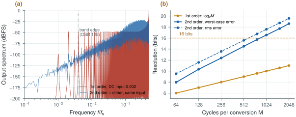
biosig.simulate_dsm() and biosig.incremental2().biosig.incremental2() runs the second-order incremental loop with \(a_1 = a_2 = 0.5\) on 8001 DC inputs across ±0.8 of full scale. Taking 16 bits to mean a worst-case error of half an LSB over the ±1 range, \(1/2^{16} = 1.5 \times 10^{-5}\):
- \(M = 512\) gives 14.5 bits, \(M = 768\) gives 15.7 bits;
- \(M = 1024\) gives 16.5 bits (largest error \(1.04 \times 10^{-5}\), which with the bound above means \(\lvert x_2\rvert_\mathrm{max} \approx 1.4\)); by rms error it is 17.6 bits.
At 500 conversions per second the loop clock is \(500 \times 1024 = 512\) kHz. A free-running third-order loop meets the same 108 dB at an OSR of 128, a clock of \(2 \times 150\ \text{Hz} \times 128 = 38.4\) kHz, more than thirteen times slower.
So the lowest clock belongs to a free-running third-order modulator, and Open-BioAFE still chooses the second-order incremental one. The reasons are the ones this chapter found. The second-order 1-bit loop is stable for any input up to full scale without NTF tuning, its reset removes idle tones and lets it be multiplexed, and its matched filter is two accumulators instead of a multi-stage decimator. The cost is clock rate. Table 14.1 lists it as a lower SQNR per OSR than a free-running ΔΣ, and Chapter 20 has to show that the integrators can run at 512 kHz within the converter’s microwatt budget.
Noise shaping makes resolution cheap in bits of hardware and expensive in clock cycles. Choose the order first: second order is robust and needs no NTF synthesis; third order and above need a synthesised NTF, a smaller input range and care with stability. Then choose the OSR from simulation, not from the formula, which is optimistic for 1-bit loops by up to 10 dB. For a multiplexed biosignal converter, the incremental form trades clock rate for reset, tone-free baselines and a trivial decimator.
ECG/EEG converter: second-order incremental ΔΣ, 1-bit quantiser, \(M = 1024\) cycles per conversion (16.5 bits worst case), 512 kHz loop clock at 500 S/s, input range ±0.8 of the reference. Reference point for comparison: a free-running third-order loop with \(\lVert\mathrm{NTF}\rVert_\infty = 1.5\) at OSR 128 (38.4 kHz).
Do not judge a modulator by the linear-model formula, or by a short simulation with a plain Hann window. The formula ignores the 1-bit quantiser’s effective gain (9 dB optimistic for the second-order loop here). A Hann window’s sidelobes leak the strongly shaped out-of-band noise of a third- or fourth-order loop back into the band and cap the measured SQNR near 100 dB; biosig.dsm_sqnr() uses a Hann² window for that reason. Simulate at several amplitudes too: a loop that is fine at −6 dBFS may be unstable at −3 dBFS.
Lab 9 synthesises first- to third-order NTFs, simulates SQNR versus OSR and the incremental mode, and designs a fixed-point CIC decimator. Start by reproducing Table 19.1 with biosig.simulate_dsm(), then redo it with python-deltasigma’s synthesizeNTF, realizeNTF and simulateDSM and compare.
Read with this chapter. Schreier, Temes and Pavan [10] for the theory, stability and incremental converters, python-deltasigma [27] for the toolbox.
- A ΔΣ loop passes the signal (STF) and high-pass filters the quantisation error (NTF); an order-\(L\) loop shapes the noise as \((2\pi f/f_\mathrm{s})^{2L}\) in band and gains \(6L + 3\) dB per octave of OSR.
- The linear model gives the slopes; simulation gives the numbers. A 1-bit second-order loop at OSR 128 reaches 85 dB at −6 dBFS, 9 dB below the formula.
- 1-bit loops above second order need \(\lVert\mathrm{NTF}\rVert_\infty \le 1.5\) (Lee criterion) and accept a smaller input; spreading the zeros across the band gains up to 11 dB.
- DC inputs make idle tones; with an ECG baseline they land in band. Higher order, dither at the quantiser and reset all cure them.
- An incremental converter resets every conversion; second order gains two bits per doubling of M and reaches 16.5 bits at M = 1024, a 512 kHz clock at 500 S/s.