Chapter 13Sampling and Quantisation
An ADC does two things to a biosignal: it looks at it only at discrete instants, and it rounds every look to one of \(2^N\) levels.
- apply the Nyquist theorem to ExG signals and predict what aliases where;
- derive the quantisation-noise model, its \(6.02N + 1.76\) dB result and its limits;
- use dither and oversampling to trade rate for resolution;
- estimate the jitter limit and see why it is minor at biosignal rates.
What sample rate and how many bits does each Open-BioAFE mode need, before any circuit is chosen?
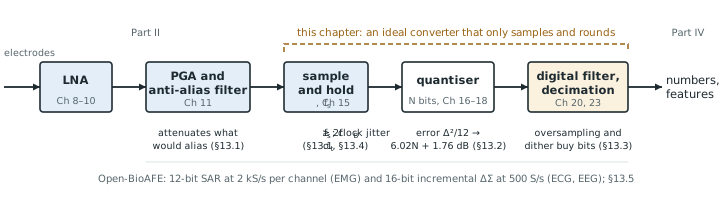
Part II ends with an amplified, filtered biosignal of a few hundred millivolts. Part III turns it into numbers. This chapter treats the converter as an ideal black box that samples and rounds, and asks only what those two operations cost. Every real converter in Chapters 15–21 adds errors on top of the ones found here, so these are the best numbers you can hope for (Figure 13.1).
13.1Sampling and aliasing with ExG examples
Sampling at a rate \(f_\mathrm{s}\) keeps one value every \(1/f_\mathrm{s}\) seconds. In the frequency domain it copies the input spectrum to every multiple of \(f_\mathrm{s}\), so after sampling there is no way to tell a tone at \(f\) from one at \(f + kf_\mathrm{s}\) or \(kf_\mathrm{s} - f\). Only the band from 0 to \(f_\mathrm{s}/2\), the Nyquist band, is unambiguous, and any input above it folds back into it:
The Nyquist theorem says that a signal confined to \(0 \ldots f_\mathrm{B}\) survives sampling if \(f_\mathrm{s} > 2f_\mathrm{B}\). The signal is rarely the problem. The trouble comes from everything else at the input that is not confined to the band: mains harmonics, EMG on an ECG lead, chopper ripple (Chapter 9), and the amplifier’s own wide-band noise. Each of these folds somewhere into the band, and once folded it cannot be filtered out.
256 S/s is a common EEG rate (Table 2.1), and its Nyquist band ends at 128 Hz. The 50 Hz fundamental and its 100 Hz harmonic are already in band and must be handled by CMRR and a digital notch. The higher harmonics fold:
- 150 Hz lands at \(\lvert 150 - 256\rvert = 106\) Hz, just above the EEG band;
- 200 Hz lands at 56 Hz, in the gamma band;
- 250 Hz lands at \(\lvert 250 - 256\rvert = 6\) Hz, in the theta band;
- 350 Hz lands at 94 Hz, and 500 Hz at 12 Hz, in the alpha band.
With 60 Hz mains, 240 Hz lands at 16 Hz and 300 Hz at 44 Hz. A 50 Hz notch filter after the converter removes none of these, and a reader of the EEG would see a narrow 6 Hz rhythm that the brain never produced.
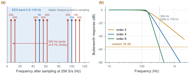
biosig.alias_freq() and biosig.butter_atten_db().An anti-alias filter in front of the sampler must therefore attenuate every interferer that could fold into the band until it is below the noise floor. The first frequency that folds into the band is \(f_\mathrm{s} - f_\mathrm{B}\), so that is where the filter has to be steep.
Sample an ECG with a 150 Hz band at 500 S/s. A tone at \(f_\mathrm{s} - f_\mathrm{B} = 350\) Hz folds onto 150 Hz. Suppose the worst interferer there is 1 mVrms, a strong EMG burst from the chest muscles. To bring it below the 1.5 µVrms noise floor the filter needs
\[A \ge 20\log_{10}\frac{1\ \text{mV}}{1.5\ \text{µV}} \approx 56\ \text{dB at 350 Hz}.\]A Butterworth low-pass with its corner at 150 Hz gives \(10\log_{10}\!\left[1 + (350/150)^{2n}\right]\): 15 dB for order 2, 29 dB for order 4, 44 dB for order 6 and 59 dB for order 8 (Figure 13.2b). An 8th-order filter with a corner set this precisely is a large analog block.
Sample at 2 kS/s instead and the first folding frequency moves to 1850 Hz, more than twelve times the band edge. A 3rd-order filter now gives 65 dB, and a digital filter after the converter removes everything between 150 Hz and 1 kHz before the rate is reduced to 500 S/s. This trade, a faster converter for a simpler analog filter, is the start of oversampling.
The lesson for a biomedical chip is that the anti-alias filter is set by the interferers, not by the signal. The ΔΣ converter of Chapter 19 samples so fast that its first folding frequency is tens of kilohertz away, where a single pole and the front-end’s own roll-off suffice; the SAR, running near the Nyquist rate, needs the filter that Chapter 11 designs.
13.2The quantisation-noise model
A converter with \(N\) bits divides its full-scale range \(V_\mathrm{FS}\) (peak to peak) into \(2^N\) steps of one LSB (least significant bit):
\[\Delta = \frac{V_\mathrm{FS}}{2^N}.\]Rounding the input to the nearest level leaves an error between \(-\Delta/2\) and \(+\Delta/2\) (Figure 13.3a). If the input is busy, crossing many levels in a way unrelated to the sampling, the error behaves like a random variable spread evenly over that interval, with a mean of zero and a power of
\[\overline{e^2} = \frac{1}{\Delta}\int_{-\Delta/2}^{\Delta/2} e^2\,de = \frac{\Delta^2}{12}.\]This is the quantisation-noise model: the quantiser is replaced by an adder that injects white noise of power \(\Delta^2/12\), spread evenly from 0 to \(f_\mathrm{s}/2\). Compare it with a full-scale sine, whose amplitude is \(V_\mathrm{FS}/2 = 2^{N-1}\Delta\) and whose power is \((2^{N-1}\Delta)^2/2\):
\[\mathrm{SQNR} = 10\log_{10}\frac{2^{2N-2}\Delta^2/2}{\Delta^2/12} = 10\log_{10}\!\left(1.5 \cdot 2^{2N}\right).\]Each bit adds 6 dB. The same relation, read backwards, defines the effective number of bits (ENOB) of a real converter: measure its signal-to-noise-and-distortion ratio and ask how many ideal bits would give the same number. A 12-bit converter with 68 dB of SNDR is an 11.0-bit converter. Chapter 14 measures SNDR properly; biosig.tone_metrics() already does it for the figures here, and quantising a near-full-scale sine with biosig.quantize() gives 74.2 dB at 12 bits and 98.4 dB at 16 bits, matching the formula.
In EMG mode the programmable gain (Chapter 11) is set so that ±5 mV at the electrodes fills the SAR’s range. Referred to the input, \(V_\mathrm{FS} = 10\) mV and a 12-bit LSB is
\[\Delta = \frac{10\ \text{mV}}{4096} = 2.44\ \text{µV}, \qquad \frac{\Delta}{\sqrt{12}} = 0.70\ \text{µVrms}.\]The analog noise in the EMG band (10–500 Hz) is about \(1.5\sqrt{490/99.5} \approx 3.3\) µVrms (Worked Example 2.3). Adding the two in power gives \(\sqrt{3.33^2 + 0.70^2} = 3.40\) µVrms: quantisation costs 2 %. A 10-bit converter would give 2.8 µVrms of quantisation noise and raise the total to 4.4 µVrms, about 30 % worse.
A useful rule follows: keep the quantisation noise at most a third of the analog noise at the converter input. Then it adds about 5 % (\(\sqrt{1 + 1/9} = 1.054\)), and more bits buy nothing.
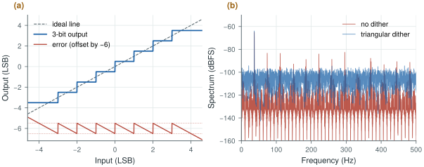
biosig.quantize().The model fails whenever the error is not busy:
- Small signals. An input that spans only a few LSB crosses the same few levels in a regular pattern, so the error is a function of the input and repeats with it. It shows up as harmonics, not noise (Figure 13.3b).
- DC and slow signals. A constant input gives a constant error, up to half an LSB of offset that no averaging removes. An ECG baseline or a slow EEG drift spends a long time near a few codes.
- Overload. Beyond full scale the error is no longer bounded at all. With an electrode offset or a motion artefact this is a real case, which is why Chapter 10 removes the offset before the converter.
The demo below shows both effects of this and the previous section. It starts at 500 S/s: push the tone above fs/2 and watch it alias, then raise the sample rate and the bits together and watch the held output close in on the tone; drop the bits to 2 or 3 and the error stops looking like noise.
13.3Dither and oversampling
The cure for a quantiser whose error is not busy is to make it busy. Adding a small random signal, dither, before the quantiser moves the input across levels at random, so the error decorrelates from the signal. Triangular dither of 1 LSB peak to peak removes the dependence of the error’s mean and power on the input entirely; Gaussian dither of about half an LSB rms or more does nearly as well. The price is the dither’s own noise, visible in Figure 13.3b as a higher floor.
A biomedical front-end usually gets dither for free. In Worked Example 13.3 the analog noise at the converter is 3.3 µVrms, which is 1.4 LSB rms. That is more than enough to keep the error white, as long as the gain stages are designed so that the amplifier’s noise, and not the quantiser, sets the floor. Choose the LSB by the one-third rule and the quantiser behaves like the model.
Once the error is white, its power \(\Delta^2/12\) is spread evenly over \(0 \ldots f_\mathrm{s}/2\). Sample faster than Nyquist and the same power is spread thinner. If the signal occupies only \(0 \ldots f_\mathrm{B}\), a digital low-pass filter after the converter keeps only the fraction \(2f_\mathrm{B}/f_\mathrm{s}\) of it. Define the oversampling ratio
\[\mathrm{OSR} = \frac{f_\mathrm{s}}{2f_\mathrm{B}}, \qquad \mathrm{SQNR} = 6.02N + 1.76 + 10\log_{10}\mathrm{OSR}\ \text{dB}.\]Every doubling of the sample rate buys 3 dB, half a bit.
A 12-bit converter samples an EEG with a 100 Hz band. At 256 S/s its SQNR is 74 dB. Run it at 25.6 kS/s instead, an OSR of 128, filter digitally and decimate back down:
\[\mathrm{SQNR} = 74.0 + 10\log_{10}128 = 74.0 + 21.1 = 95.1\ \text{dB} \;\approx\; 15.5\ \text{bits}.\]Four extra bits, but at a hundred times as many conversions, and so roughly a hundred times the converter energy. And it works only if the error is white: the simulated points in Figure 13.4a fall up to 3 dB short at high OSR because a pure sine’s quantisation error has harmonics that stay in band.
A noise-shaping loop does far better at the same OSR. With a 1-bit quantiser, plain oversampling by 128 gives only 29 dB; a second-order noise-shaping loop gives about 100 dB in the linear model of Chapter 19 and 85 dB in simulation at −6 dBFS, because it pushes the quantisation noise out of the band instead of only spreading it.
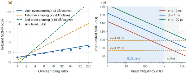
biosig.sqnr_os_db() and biosig.jitter_snr_db().13.4Clock jitter
A sampling clock whose edges wander by \(\sigma_t\) rms samples the input at slightly wrong instants. For a sine of amplitude \(A\) at \(f_\mathrm{in}\) the error is the slope times the timing error, at most \(2\pi f_\mathrm{in} A\,\sigma_t\), and comparing its rms value with the signal’s gives
The limit depends on the input frequency, and biosignals are slow.
For the 16-bit ΔΣ channel, 98 dB at the top of the ECG band (150 Hz) needs
\[\sigma_t < \frac{1}{2\pi \cdot 150\ \text{Hz} \cdot 10^{98/20}} \approx 13\ \text{ns}.\]For the 12-bit SAR in spike mode, 74 dB at 7 kHz needs \(\sigma_t < 4.5\) ns. In EMG mode, 1 ns of jitter at 500 Hz limits the SNR to 110 dB, far above anything the channel can use.
Nanoseconds of jitter are easy: an on-chip relaxation or ring oscillator with period jitter far below a nanosecond costs microwatts. This is the opposite of the SerDes world, where femtoseconds matter [3]. A biomedical converter worries about energy per conversion instead, which is the subject of Chapter 14. The one exception is the continuous-time ΔΣ modulator, whose feedback DAC turns clock jitter into a noise source of its own (Chapter 20).
13.5Rates and bits for each mode
The answer to the design question combines the bands of Chapter 2, the dynamic range of Worked Examples 2.2 and 2.3 and the anti-alias trade of this chapter.
Table 13.1. Output rate and resolution for each Open-BioAFE mode. The output rate is after any decimation. “Bits needed” comes from the dynamic range over the analog noise in the mode’s band.
| Mode | Band | Converter | Output rate | Bits needed | Why |
|---|---|---|---|---|---|
| ECG | 0.05–150 Hz | Incremental ΔΣ | 500 S/s | 16 (up to 17 DC-coupled) | 103 dB with the full ±300 mV offset; less after the DC servo loop |
| EEG | 0.5–100 Hz | Incremental ΔΣ | 256–500 S/s | 16 | Same offset problem, smallest signals |
| EMG | 10–500 Hz | SAR | 2 kS/s | 10–11 (12 built) | 60–67 dB AC-coupled; the one-third rule gives 12 |
| Spikes (optional) | 0.3–7 kHz | SAR | 20–30 kS/s | 8–10 | About 30 dB of spike over wide-band noise, plus margin for LFP and artefacts |
The two Nyquist-rate SAR modes run at three to four times their band edge, so the analog filter of Chapter 11 can be of modest order. The ΔΣ modes run their modulator far faster, at an OSR that Chapter 19 chooses, and decimate down to the rates in the table.
Choose the sample rate from the interferers you must keep out of the band, not from the signal: the faster you sample, the simpler the analog filter and the more the digital filter does. Choose the bits so that quantisation noise is at most a third of the analog noise; beyond that, bits are wasted energy. Jitter is not a concern at ExG rates, so the clock can be a cheap on-chip oscillator.
ECG and EEG: 16-bit incremental ΔΣ, 256–500 S/s output. EMG: 12-bit SAR at 2 kS/s. Spikes (optional): the same SAR at 20–30 kS/s. Sampling-clock jitter below 1 ns rms.
A 50 Hz notch filter after the converter does not remove mains interference that has already aliased. If a mains harmonic folds into the band, it appears at a frequency the notch does not touch, such as 6 Hz in Worked Example 13.1. Filter before sampling, or sample fast enough that the harmonics have somewhere harmless to fold.
Lab 6 quantises sine waves, applies coherent sampling and windows, and builds the adctest.py module every later converter lab uses. Start from biosig.quantize() and biosig.tone_metrics(), then reproduce Figure 13.3 and the 6.02N + 1.76 dB line.
Read with this chapter. Pelgrom [9] for sampling, quantisation and jitter, Schreier, Temes and Pavan [10] for oversampling and the noise model.
- Sampling folds everything above \(f_\mathrm{s}/2\) into the band; the anti-alias filter is set by the interferers, which fold to frequencies no later filter can reach.
- At 256 S/s the 250 Hz mains harmonic lands at 6 Hz; a Nyquist-rate ECG channel at 500 S/s needs an 8th-order filter for a 1 mVrms interferer, while 2 kS/s needs only 3rd order.
- An ideal \(N\)-bit quantiser gives \(6.02N + 1.76\) dB with a full-scale sine; the white-noise model fails for small, slow or overloading inputs, and dither (often the front-end’s own noise) restores it.
- Keep quantisation noise at most a third of the analog noise; for EMG that means 12 bits over ±5 mV.
- Plain oversampling buys only 3 dB per octave; noise shaping (Chapter 19) does much better.
- Jitter of a few nanoseconds is harmless at ExG frequencies.