Open-SERDES introduction talk
Intro Slides
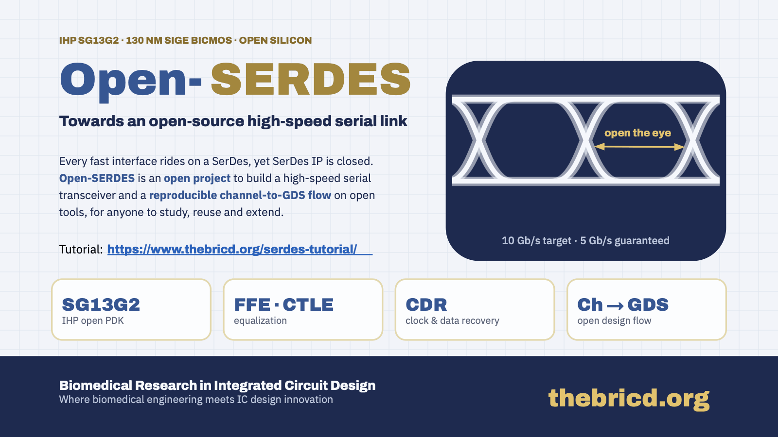
The talk that introduces Open-SERDES: why an open serial link, why IHP SG13G2, the anatomy of the link, the open channel-to-GDS flow, what we will build and test, and the roadmap. Speaker notes sit under each slide; the tutorial chapter that goes deeper is linked where there is one.
These slides were prepared with the help of AI tools and may contain mistakes. If you find one, please email bricd.org@gmail.com and we will correct it.
Speaker notes
Close on the call to action: Open-SERDES is an open BRICD project. We are looking for contributors and collaborators at every level, from link modeling to layout and measurement. Contact: kithminr@uom.lk, thebricd.org. Thank the audience and invite questions.
Speaker notes
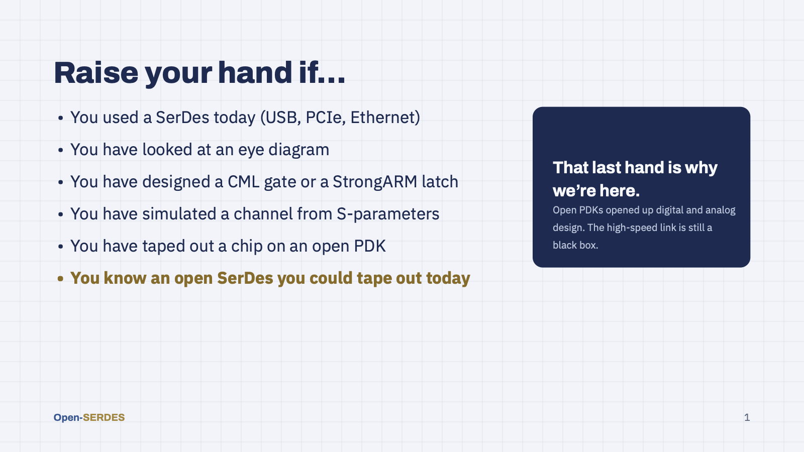
Icebreaker, borrowed from the FSiC format. Expect many hands for the first two, fewer for CML/StrongARM and S-parameters, some for open-PDK tapeouts, and essentially none for the last one. That silence is the motivation for the whole project.
Speaker notes
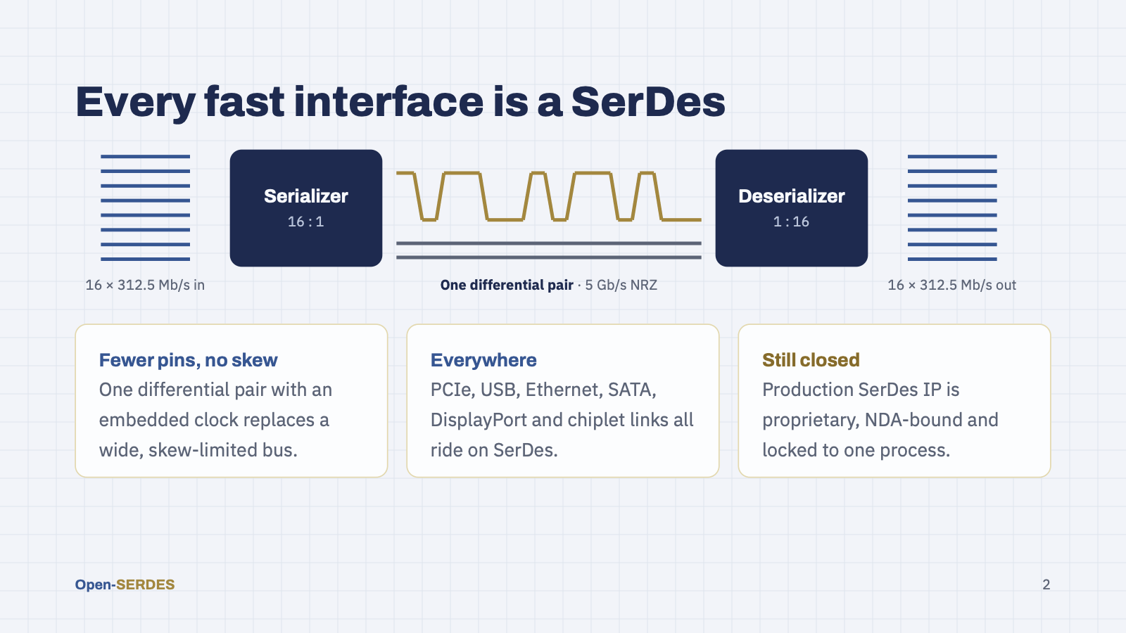
A SerDes turns a wide, slow parallel bus into one fast serial stream and back. Example numbers: 16 lanes at 312.5 Mb/s become a single 5 Gb/s NRZ stream on one differential pair. That is why every modern high-speed interface uses one. The catch: every production SerDes is closed IP, so almost nobody outside a handful of companies ever sees a complete design.
Speaker notes
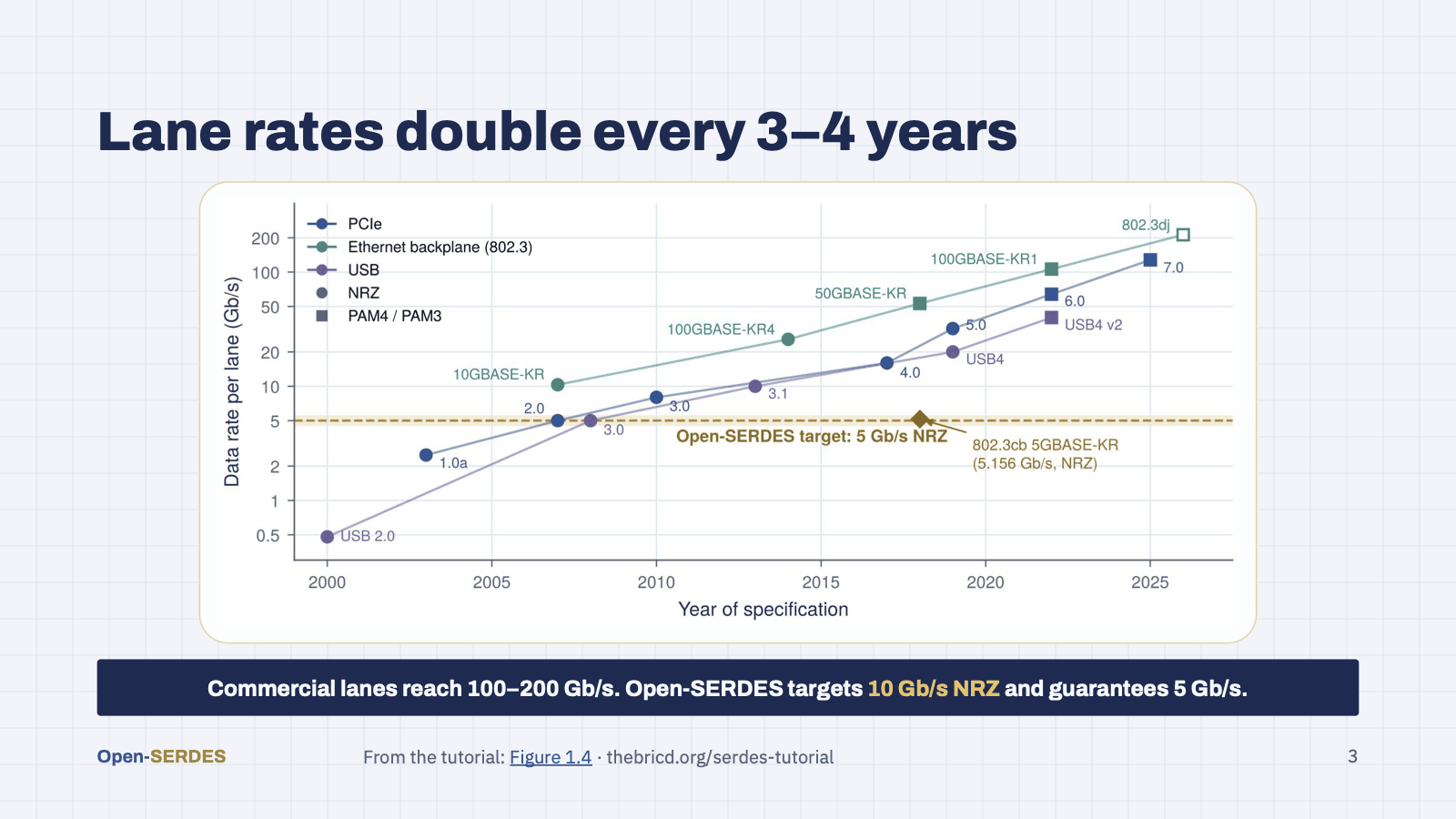
Per-lane rates have doubled every three to four years: PCIe, backplane Ethernet and USB all climb the same line, and commercial lanes now reach 100 to 200 Gb/s. We start low on that curve on purpose. Every high-speed block is designed for 10 Gb/s NRZ, the 10GBASE-KR and SFP+ class, and 5 Gb/s, the PCIe 2.0 and 5GBASE-KR class, is the guaranteed mode of first silicon: hard enough to need equalization and clock recovery, modest enough for a first tapeout on an open PDK. Figure 1.4 of the tutorial.
Speaker notes
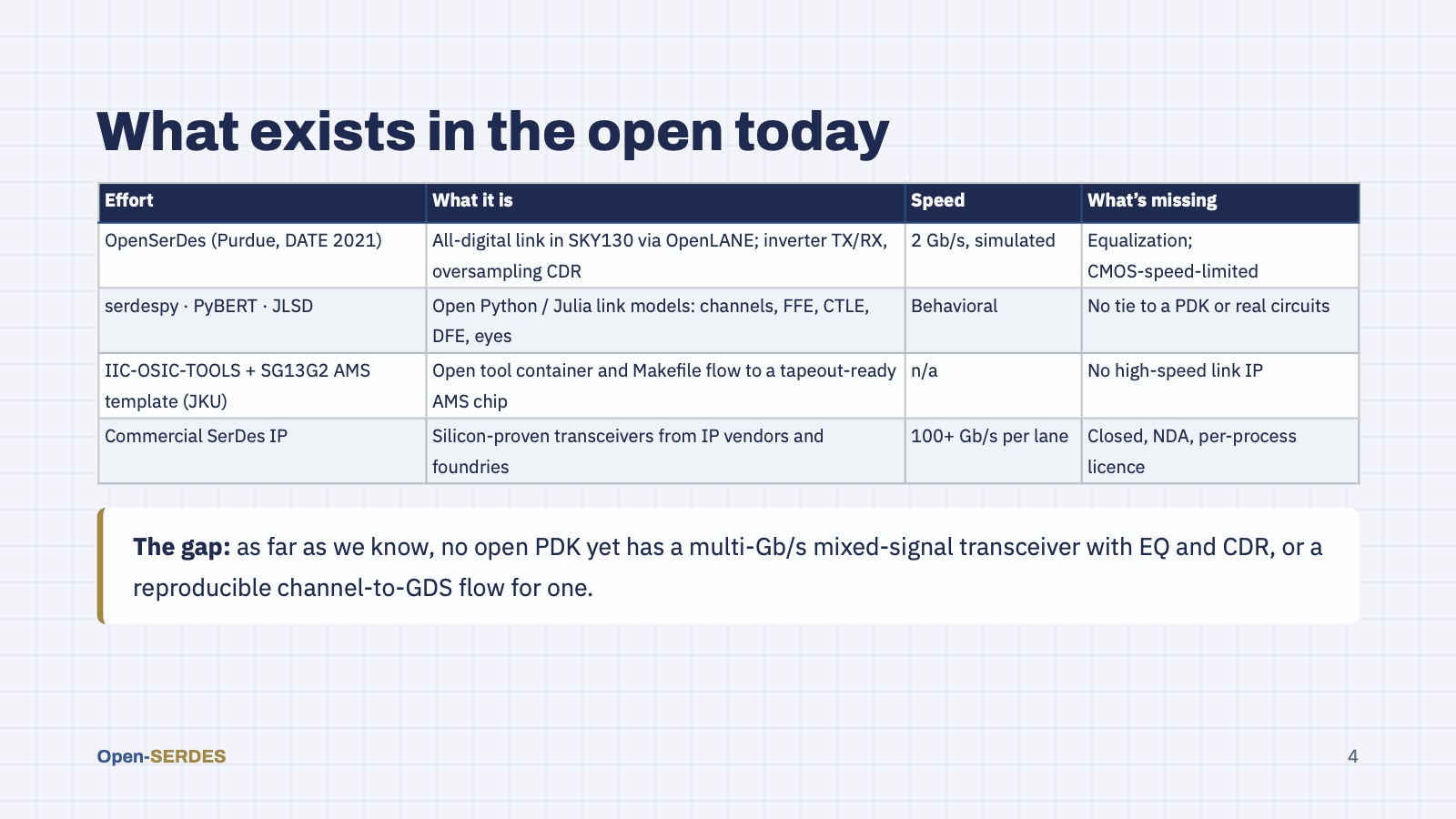
Be fair to prior work. Purdue’s OpenSerDes (Kumar, Chatterjee, Sen, DATE 2021) is the closest: a fully synthesizable all-digital link in SKY130 at 2 Gb/s in post-layout simulation, about 438 mW including SER/DES/CDR, with no equalization. The Python and Julia link simulators are excellent but live at the system level. JKU’s template gives us the flow. Nobody has yet put these together into a mixed-signal, equalized, multi-Gb/s link on an open PDK. That is the gap Open-SERDES targets.
Speaker notes
Part 1: the process. Why we chose IHP’s open SiGe BiCMOS PDK, and the SG13G2 work we already have.
Speaker notes
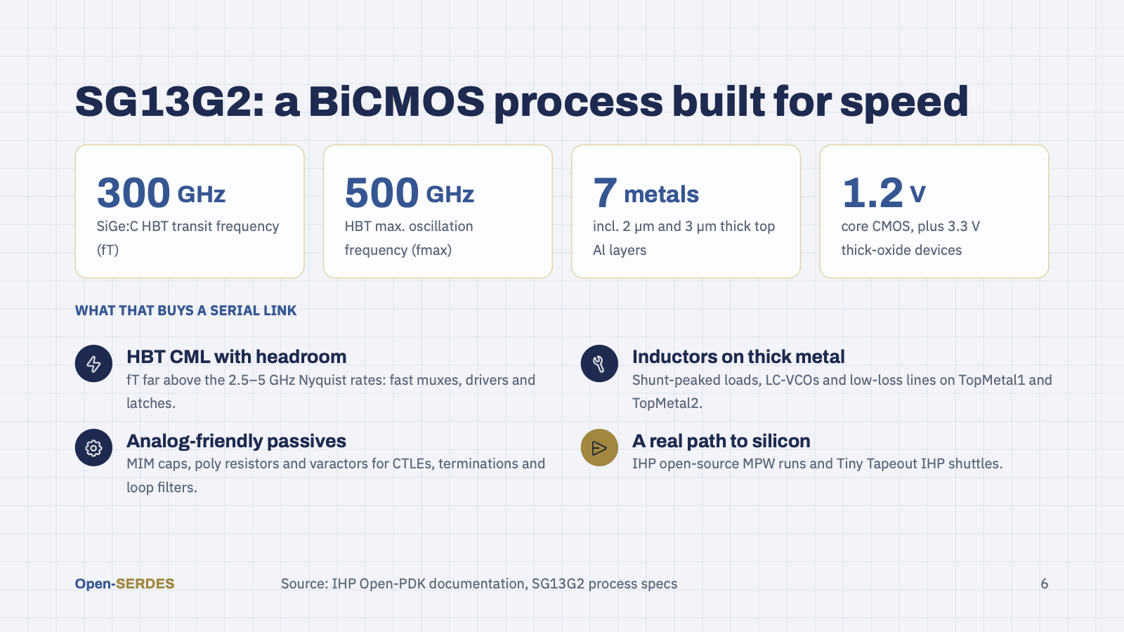
SG13G2 is IHP’s high-performance 130 nm SiGe:C BiCMOS. The PDK documentation lists HBTs with about 300 GHz fT and 500 GHz fmax (IHP’s MOS-AK 2025 talk quotes 350 / 450 GHz, with BVceo of 1.6 V). For 5 Gb/s NRZ the Nyquist frequency is only 2.5 GHz, and even the 10 Gb/s target needs only 5 GHz, so HBT current-mode logic has enormous headroom; that is exactly what the 130 nm SKY130 CMOS designs lacked. Seven aluminium layers, the top two 2 µm and 3 µm thick, give us decent inductors and lines. And, crucially, there is an open MPW path, including Tiny Tapeout on IHP.
Speaker notes
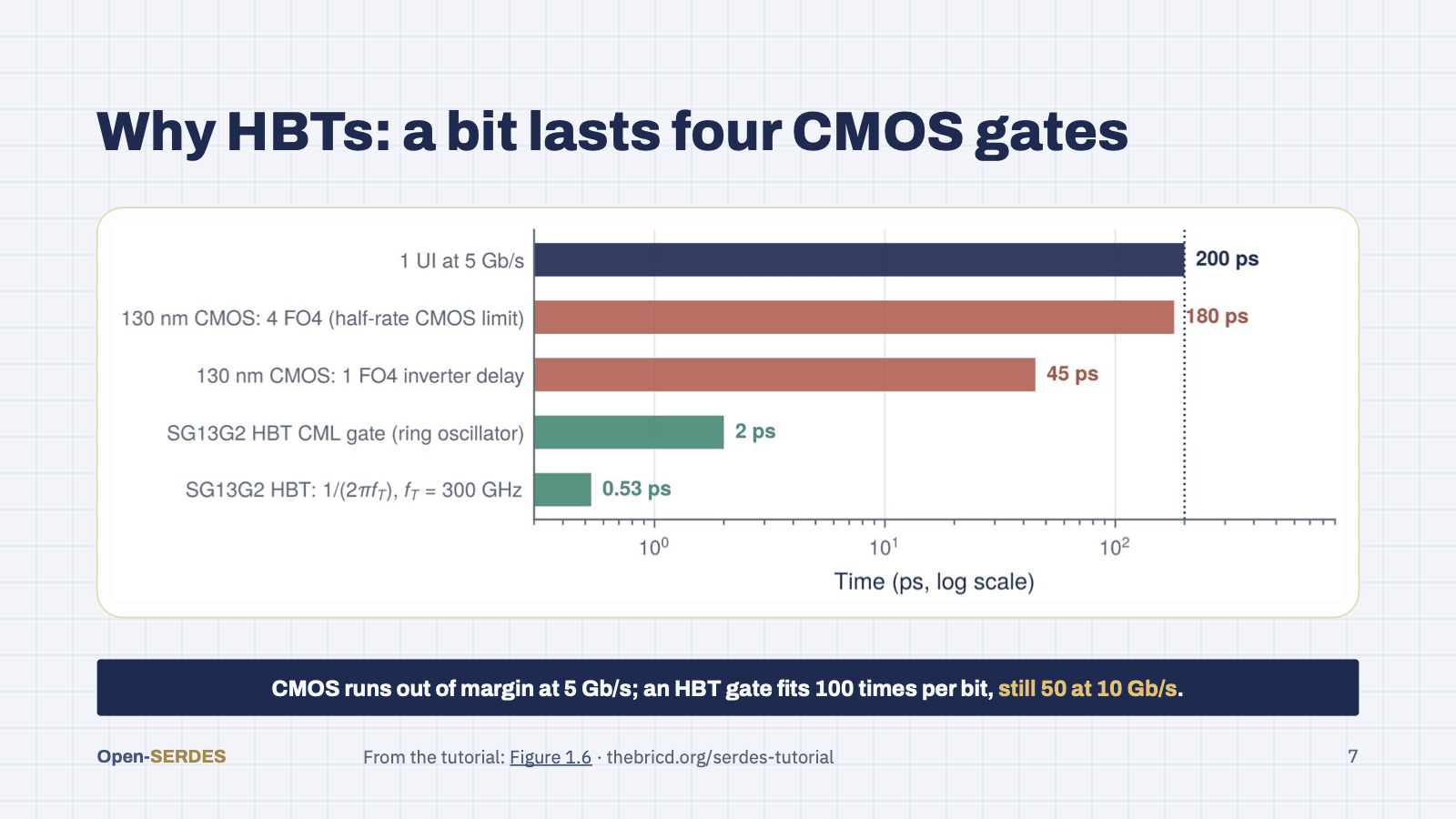
This is the case for SG13G2 in one picture. Half-rate CMOS needs roughly three to four FO4 delays per bit, and 130 nm CMOS fits about four into a 200 ps UI, so it has almost no margin at 5 Gb/s. An SG13G2 CML gate is about 2 ps in a ring oscillator; even loaded, it fits many times over. Even a 100 ps bit at the 10 Gb/s target holds about fifty HBT gate delays. So the design rule is HBT CML wherever a signal runs at 1.25 GHz or faster, and CMOS everywhere else. Figure 1.6 of the tutorial.
Speaker notes
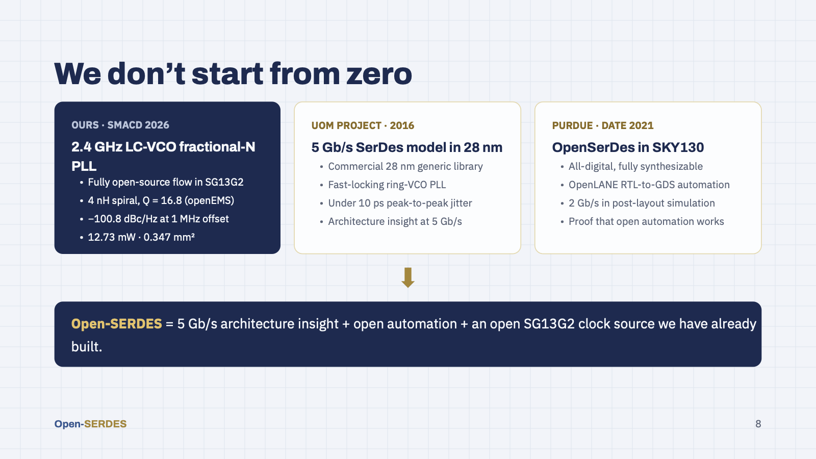
Three threads come together. First, our own open SG13G2 PLL, accepted at SMACD 2026: a 2.4 GHz type-II fractional-N PLL with a cross-coupled LC-VCO and a custom 4 nH spiral (Q of 16.8, modelled in openEMS), −100.8 dBc/Hz at 1 MHz, 12.73 mW, 0.347 mm². A half-rate 5 Gb/s link needs a 2.5 GHz clock, right next door; for the 10 Gb/s target the VCO moves to 10 GHz with a divide-by-2 for I and Q, and the loop design and the open flow carry over. Second, an earlier University of Moratuwa project modelled a 5 Gb/s SerDes in a commercial 28 nm library, with a fast-locking ring-VCO PLL under 10 ps peak-to-peak jitter. Third, Purdue showed that open RTL-to-GDS automation can produce a working link. Open-SERDES combines all three on a faster, open BiCMOS node.
Speaker notes
Part 2: the link itself. What blocks a serial link needs, what 5 Gb/s means in numbers, and which architectural choices are still open.
Speaker notes
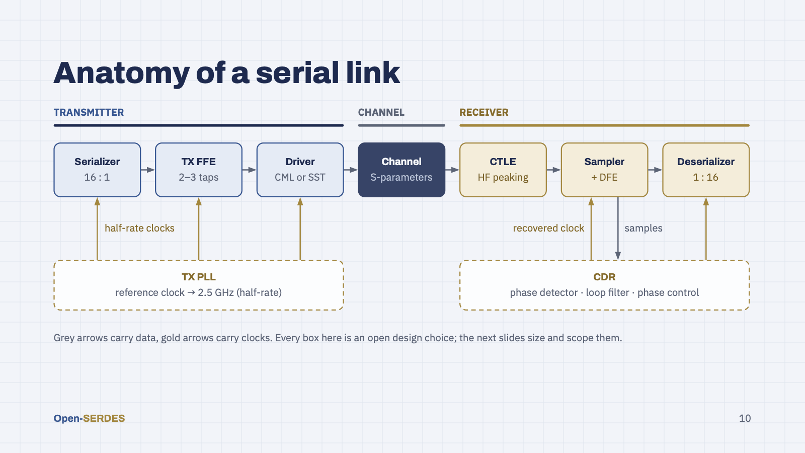
Walk the link left to right. TX: a 16:1 serializer (a mux tree whose last stage runs at the full rate), a 2–3 tap feed-forward equalizer to pre-distort against channel loss, and a driver, current-mode (CML) or voltage-mode (SST), into a 100 Ω differential line. The channel is package, PCB traces and connectors, characterized by S-parameters. RX: a CTLE boosts high frequencies, a sampler (optionally with a DFE) decides bits, and the deserializer fans them back out. Clocking is the hard part: a TX PLL generates the half-rate 2.5 GHz clocks; on the RX side a CDR extracts timing from the data itself and steers the sampling phase.
Speaker notes
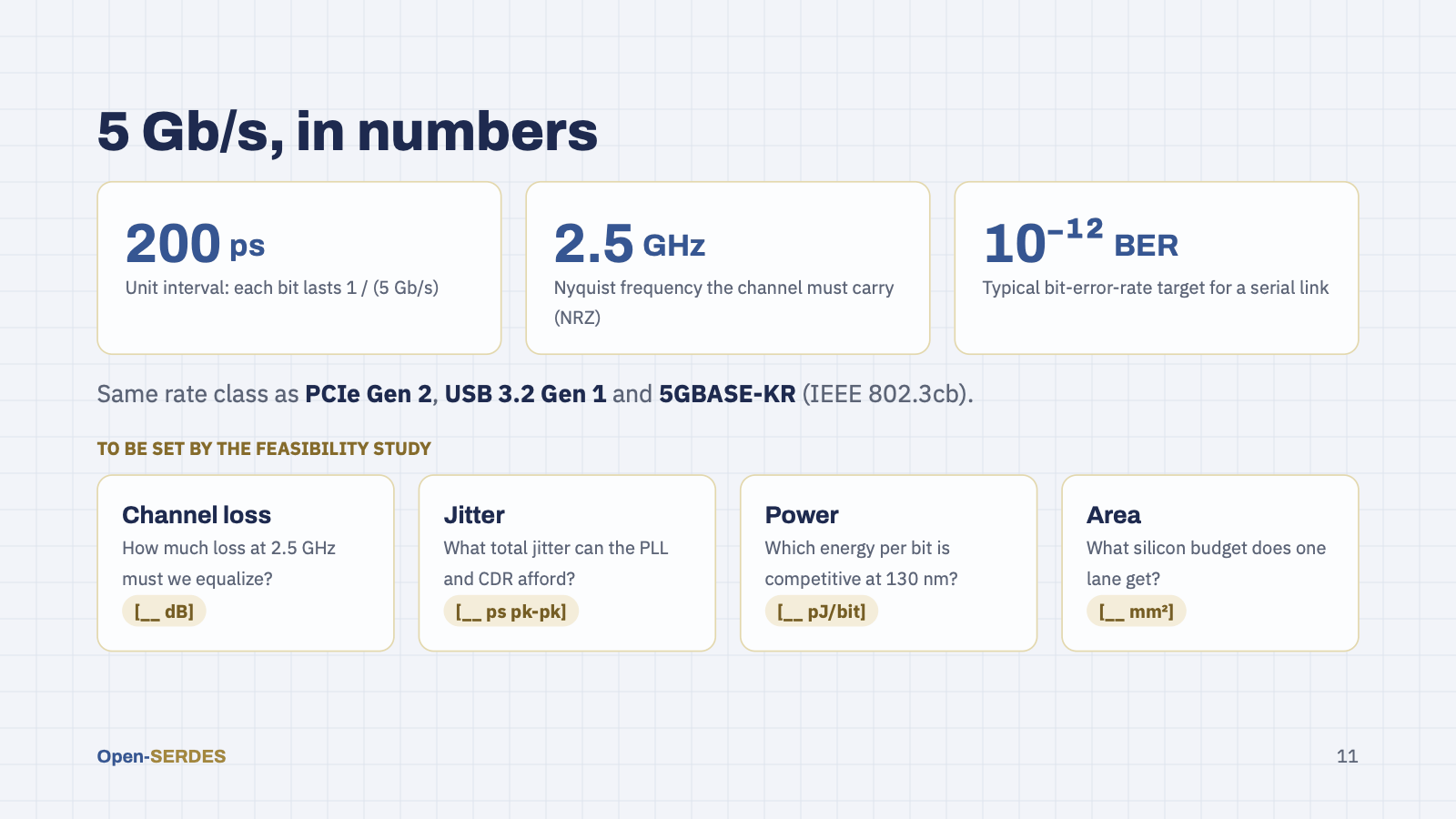
At 5 Gb/s NRZ each bit lasts 200 ps and the channel has to carry energy up to the 2.5 GHz Nyquist frequency. A BER of 1e-12 or better is the usual serial-link target. This is the same rate class as PCIe Gen 2, USB 3.2 Gen 1 and 5GBASE-KR backplane Ethernet, so standard channel models exist to test against. For the 10 Gb/s design target the bit time halves to 100 ps and the Nyquist frequency doubles to 5 GHz. The bracketed numbers are deliberately open: the first deliverable of the project is a feasibility study that fixes the channel, jitter, power and area budgets.
Speaker notes
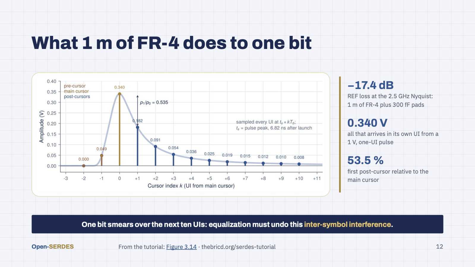
REF is the reference channel used throughout the tutorial: one meter of FR-4 with 300 fF pads, losing 17.4 dB at the 2.5 GHz Nyquist frequency. Send it a single 1 V bit and only 0.34 V arrives in that bit's own UI; the rest smears into the bits that follow. The first post-cursor alone is more than half the main cursor. Every equalizer in this project exists to clean up that tail. Figure 3.14 of the tutorial.
Speaker notes
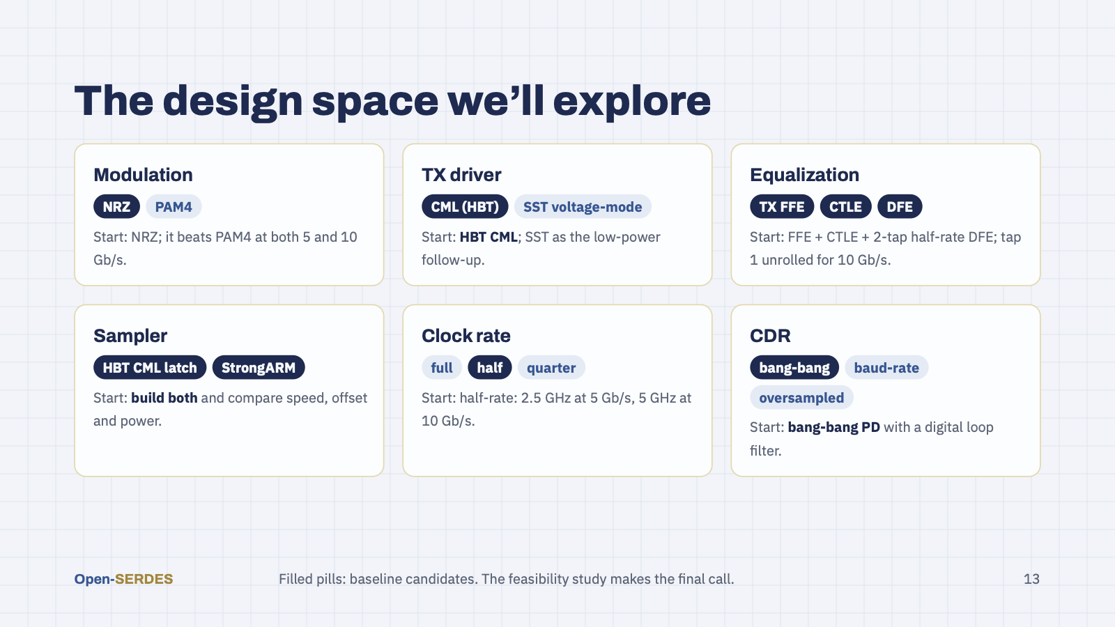
This is where we want community input. Our current baseline: NRZ, because at 5 and at 10 Gb/s PAM4 costs SNR and receiver complexity for no real gain. An HBT current-mode driver, since SG13G2’s bipolars make CML fast and robust; a source-series-terminated voltage-mode driver is the low-power alternative. A 2–3 tap TX FFE, an RX CTLE and a 2-tap half-rate DFE: the split the tutorial's equalization study recommends for the reference channel (more taps only if a harder channel needs them). For the sampler we want to build both an HBT CML latch and a CMOS StrongARM and compare them. Half-rate clocking means a 2.5 GHz clock at 5 Gb/s, very close to our existing 2.4 GHz LC-PLL, and 5 GHz at the 10 Gb/s target, from a 10 GHz VCO and a divide-by-2. At 10 Gb/s the 100 ps bit is shorter than the tap-1 feedback loop, so tap 1 of the DFE is unrolled. And a bang-bang (Alexander) phase detector with a digital loop filter, the most robust CDR to get working first; baud-rate Mueller–Müller and oversampled CDRs are alternatives.
Speaker notes
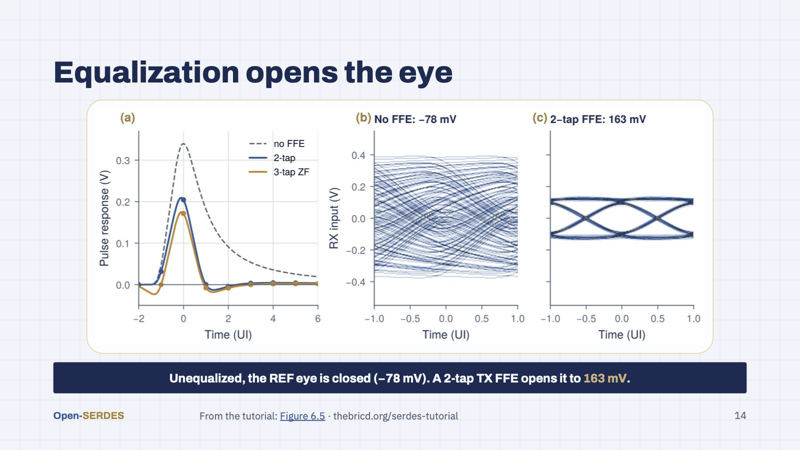
Left, the REF pulse response with and without a TX FFE; middle and right, PRBS7 eyes at the receiver input on the same scale. Without equalization the eye is closed: the worst-case patterns overlap by 78 mV. A 2-tap FFE opens it to 163 mV. The price is swing: transmit equalization takes energy away, so the open eye is only about a third of the unequalized swing. That is why the job is shared between the TX, the CTLE and the DFE. Figure 6.5 of the tutorial.
Speaker notes
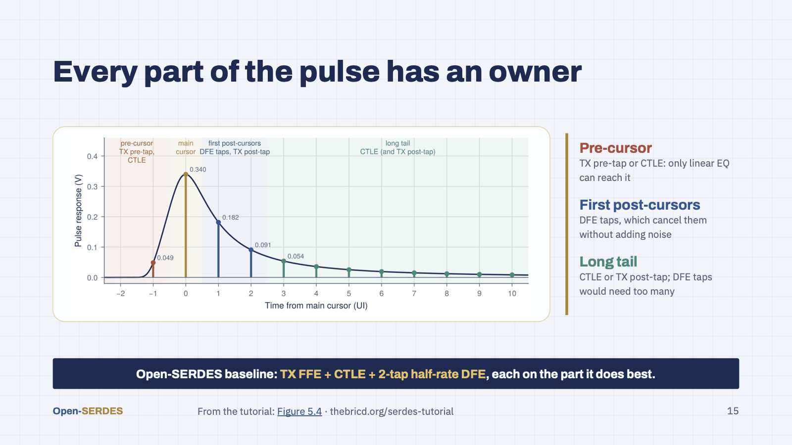
The pulse response tells you who should do what. The pre-cursor arrives before the bit is decided, so only a linear equalizer can remove it: the TX pre-tap or the CTLE. The first post-cursors are the DFE's job, and the DFE removes them without amplifying noise. The long tail would need many DFE taps, so the CTLE or the TX post-tap flattens it instead. That division of labor is the Open-SERDES baseline. Figure 5.4 of the tutorial.
Speaker notes
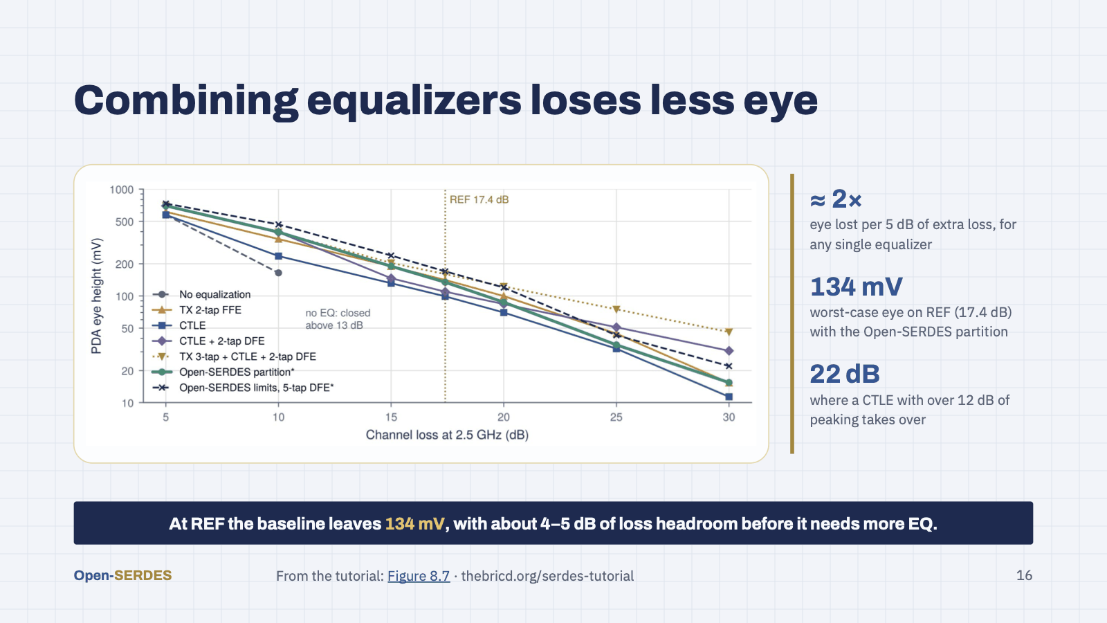
Each curve is the worst-case (peak-distortion) eye against channel loss at Nyquist, on a log scale. Every single strategy loses about a factor of two in eye per 5 dB of loss; combinations lose less. At REF the Open-SERDES partition, FFE plus CTLE plus a 2-tap DFE, leaves 134 mV. Above about 22 dB a CTLE with more than 12 dB of peaking overtakes it, which is the signal that a lossier channel would need more equalization. Figure 8.7 of the tutorial.
Speaker notes
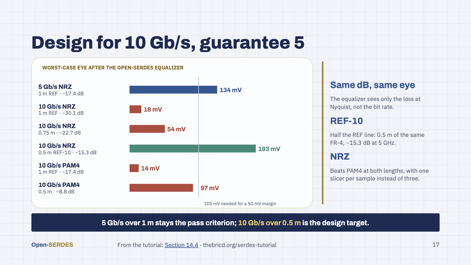
Can the same architecture go faster? We re-ran the tutorial's equalization study with the bit rate as a variable. The equalizer only sees the loss at the Nyquist frequency: over the full 1 m reference channel, 10 Gb/s meets 30 dB of loss and the worst-case eye closes to 18 mV. Over half the line, 0.5 m with the same pads, which we call REF-10, it opens to 193 mV, more than our 5 Gb/s baseline gets over 1 m. PAM4 does worse than NRZ at both lengths and needs three slicers per sample. So the plan is: design every high-speed block for 10 Gb/s, and keep 5 Gb/s over the 1 m channel as the pass criterion of first silicon. Section 14.4 of the tutorial.
Speaker notes
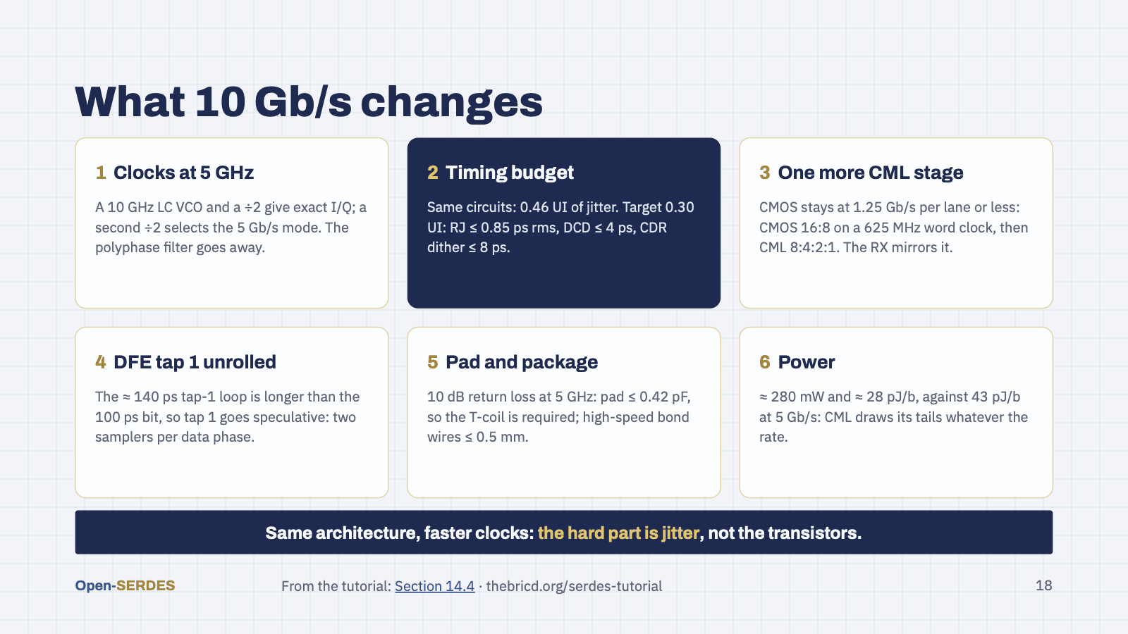
What does 10 Gb/s cost? The block diagram stays; six things change. The half-rate clock doubles to 5 GHz, best made with a 10 GHz LC VCO and a divide-by-2, which also gives exact I and Q and a rate select. The timing budget is the real work: with the same circuits, jitter would take 0.46 UI, so every picosecond term must roughly halve, down to 0.85 ps rms of random jitter. One more CML mux and demux stage keeps CMOS at 1.25 Gb/s per lane. The DFE's tap-1 loop no longer fits in one bit, so tap 1 is unrolled. The pad needs the T-coil and bond wires of half a millimetre. And power rises only to about 280 mW, so energy per bit falls to about 28 pJ/b.

Speaker notes
Part 3: the workflow. This is the real contribution: a design and simulation flow anyone can rerun, from a channel S-parameter file all the way to a tapeout-ready GDS.
Speaker notes
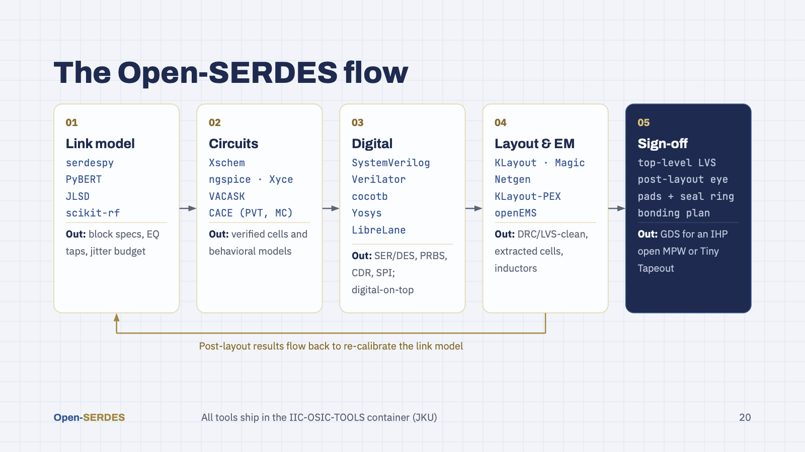
Five stages. One: a system-level link model in Python or Julia (serdespy, PyBERT, JLSD, with scikit-rf for S-parameters) turns a channel into block specifications: EQ taps, CTLE peaking, jitter budget. Two: transistor-level design in Xschem with ngspice, Xyce or VACASK, and CACE for PVT corners and Monte Carlo. Three: the digital side (serializer, deserializer, PRBS generator and checker, CDR loop logic) in SystemVerilog, verified with Verilator and cocotb, hardened with Yosys and LibreLane as part of the chip, digital-on-top, rather than as separate macros. Four: custom layout in KLayout or Magic, LVS with Netgen, parasitic extraction, and openEMS for inductors and pads. Five: top-level sign-off and a GDS ready for an IHP open MPW or Tiny Tapeout. The orange loop is the key idea: extracted results go back into the link model, so the model stays honest.
Speaker notes
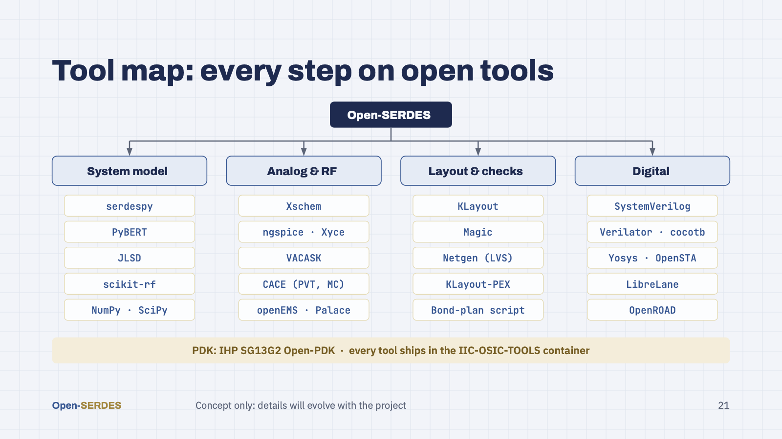
Mirrors the IIC-OSIC-TOOLS overview: one open tool, or a small set of alternatives, for each stage of the Open-SERDES flow. All of them run inside the IIC-OSIC-TOOLS container with the IHP SG13G2 Open-PDK.
Speaker notes
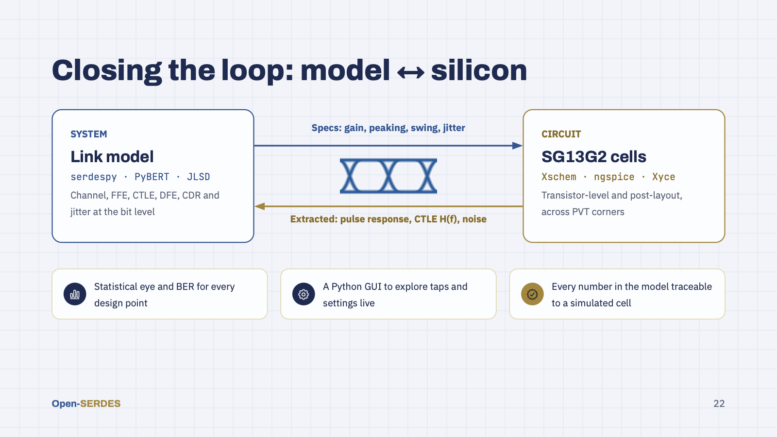
This is the piece nobody has in the open today. System-level link simulators are usually driven by idealized numbers; circuit designers work against specs handed to them. We want both directions automated: the link model generates block specs (gain, CTLE peaking, output swing, jitter allocations), and the circuit flow returns extracted pulse responses, CTLE transfer functions and noise that are dropped straight back into the model. The outcome is a statistical eye and BER for each design point, a Python GUI in the spirit of JLSD for exploring settings, and a model whose every number traces back to a simulated, and later measured, SG13G2 cell.
Speaker notes
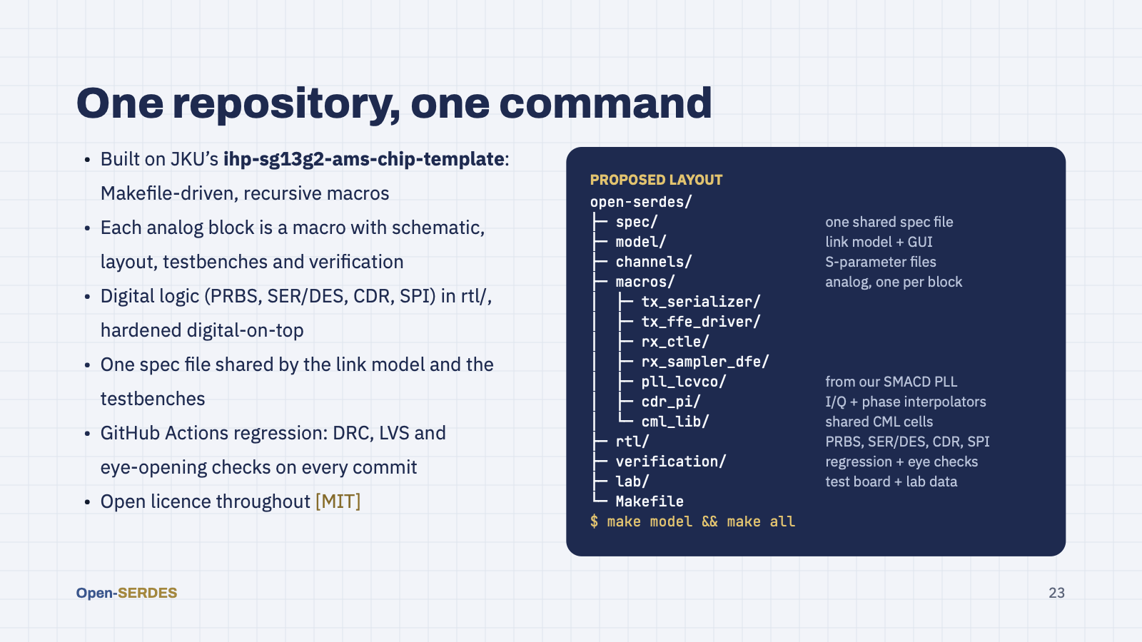
We do not want to reinvent the project infrastructure. Simon Dorrer and Harald Pretl’s ihp-sg13g2-ams-chip-template already gives a Makefile-driven, recursive macro structure that goes to a tapeout-ready chip with one make all. Open-SERDES keeps that layout: every analog block is a macro with its own schematics, testbenches, layout, verification and Makefile, so it can be built and checked on its own, and cml_lib holds the shared HBT CML cells. The digital half (PRBS, the CMOS serializer and deserializer stages, the CDR loop filter and SPI) is not a macro: it lives in rtl/ and is hardened with the chip, digital-on-top. Open-SERDES adds four folders of its own: spec, model, channels and lab. The key addition is the single spec file in spec/, read by the Python model and by every testbench, plus continuous-integration checks that include eye opening, not only DRC and LVS. The licence is still to be confirmed.
Speaker notes
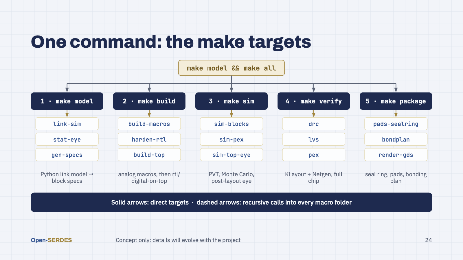
Mirrors the JKU template Makefile tree as the Open-SERDES repository uses it (Section 15.4.1 of the tutorial). make model runs the link model first; make all then builds, simulates and verifies every analog macro, hardens the rtl/ logic with the chip, digital-on-top, and packages the chip with its seal ring, pads and bonding plan. build, sim and verify recurse into every macro folder, which all expose the same targets, so each block can also be built and tested on its own.
Speaker notes
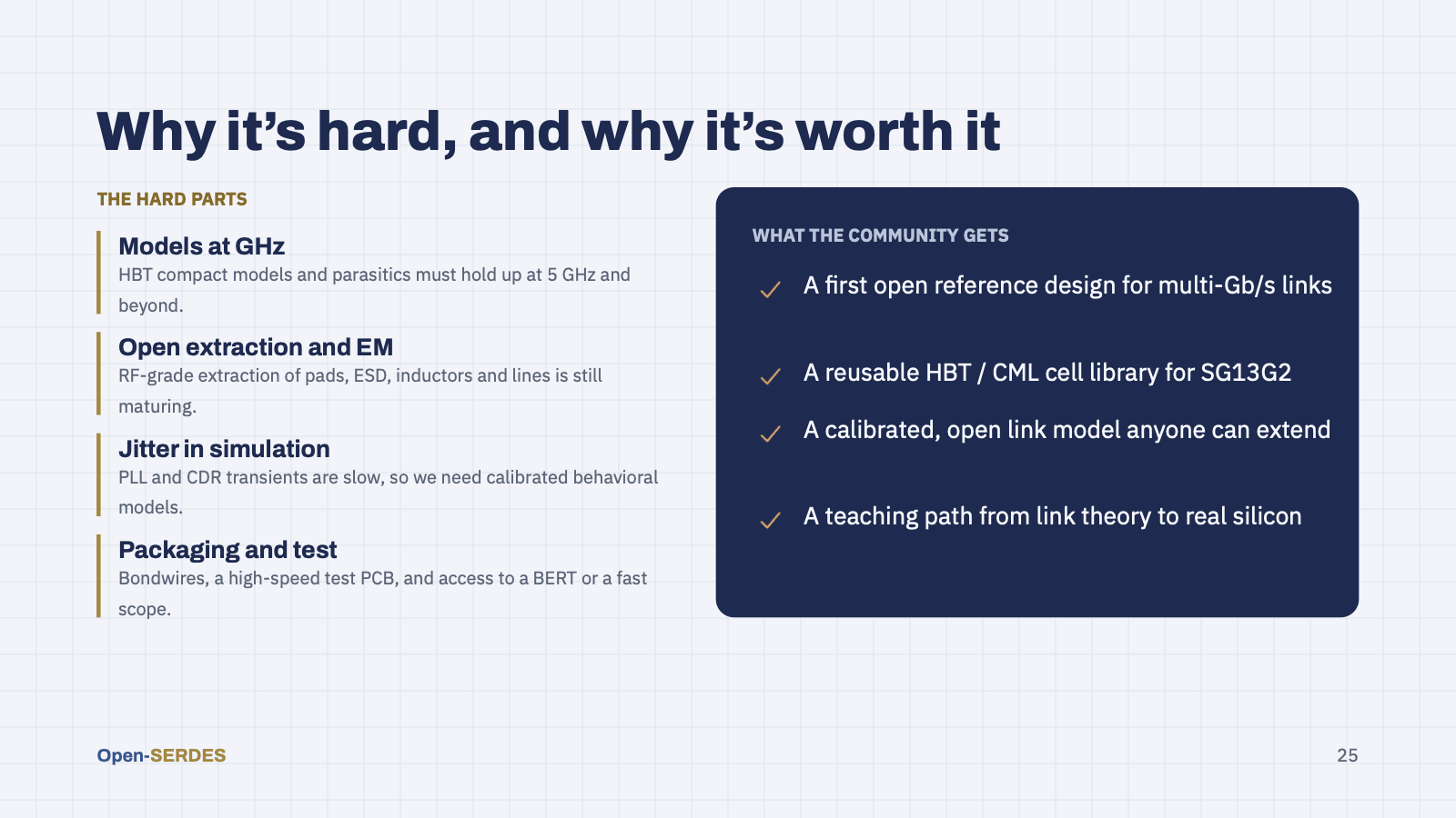
Be honest about the risk. At these speeds the weak points are model accuracy (HBT compact models and layout parasitics at multi-GHz), the maturity of open RF extraction and EM tools for pads, ESD structures and inductors, simulation time for PLL and CDR loops, and the very practical problem of packaging and measuring a 5 to 10 Gb/s signal. Each of those is also a contribution in its own right. If we succeed, the community gets the first open multi-Gb/s reference design, a reusable CML cell library, a calibrated link model, and a complete teaching path from textbook link theory to silicon.
Speaker notes
Part 4: what we will actually deliver, what the chip looks like, and how we will test it, in simulation and in the lab. Everything here is a concept and will evolve.
Speaker notes
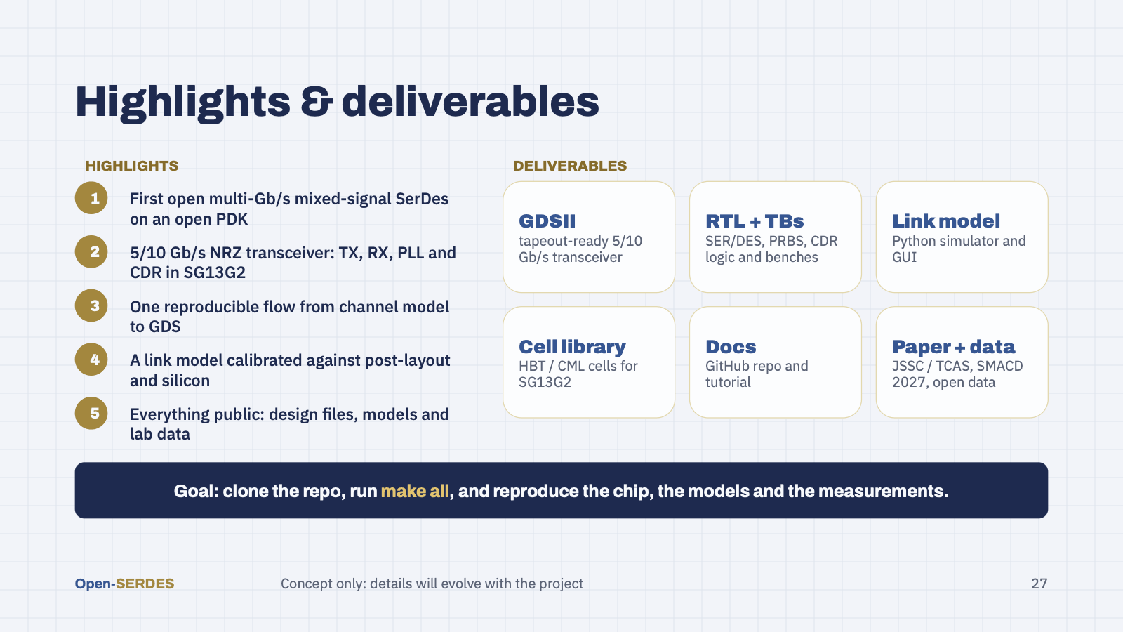
The A-to-Z summary. Highlights: what makes the project new. Deliverables: what anyone will be able to download at the end: the GDS, the RTL and benches, the link model with its GUI, a reusable HBT/CML cell library, documentation, and the paper with open measurement data.
Speaker notes
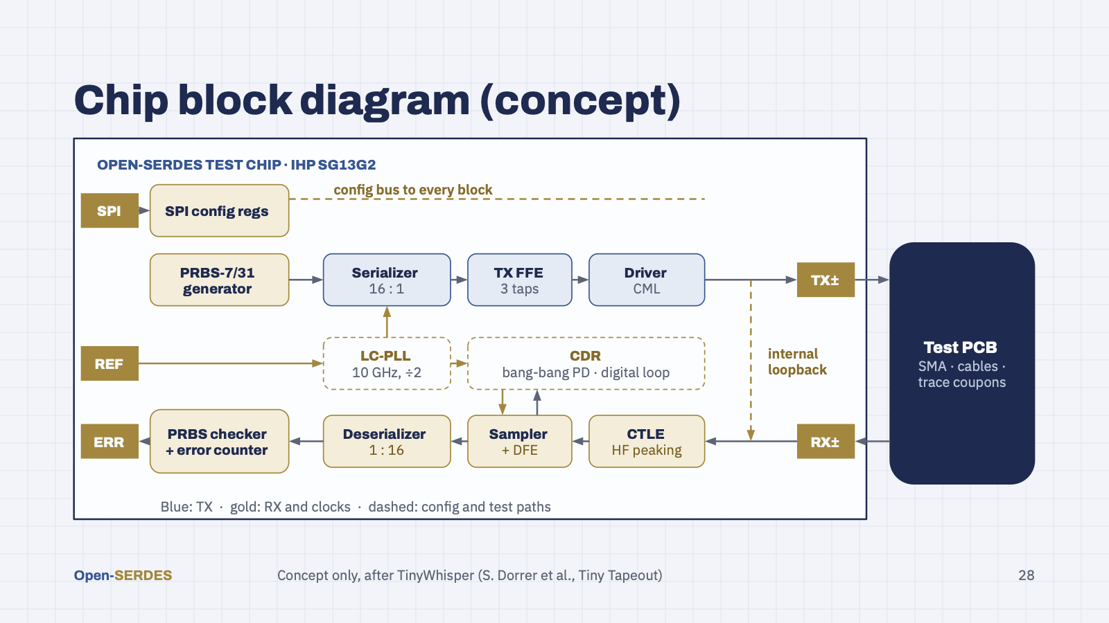
One possible test chip, in the spirit of the TinyWhisper block diagram. Digital on the left: SPI configuration registers, a PRBS-7/31 generator and a PRBS checker with error counter. TX on top: serializer, FFE and driver to the TX pads. RX below: CTLE, sampler with optional DFE, and deserializer back to the checker. The LC-PLL (a 10 GHz VCO with dividers, so one register selects 5 or 10 Gb/s) takes an external reference and clocks the TX; the CDR recovers timing for the sampler. An internal loopback lets us test TX into RX on chip, and the external test PCB closes the loop through a real channel. An external clock input lets both modes be measured without the on-chip PLL.
Speaker notes
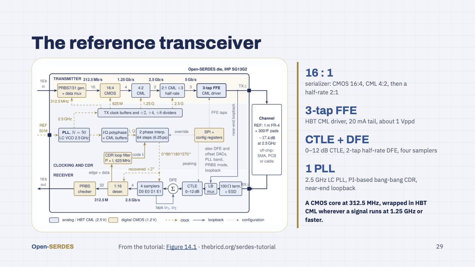
This is the 5 Gb/s reference design the tutorial builds up to; the 10 Gb/s target keeps it and changes the six things listed under 'What 10 Gb/s changes'. Read the transmitter band left to right and the receiver band right to left. The core is CMOS at 312.5 MHz; everything at 1.25 GHz or faster is HBT CML. One 2.5 GHz PLL is used twice: divided down for the TX, and split into I and Q and rotated by phase interpolators for the RX. The CDR is a digital loop, and a near-end loopback lets the chip test itself. Figure 14.1 of the tutorial.
Speaker notes
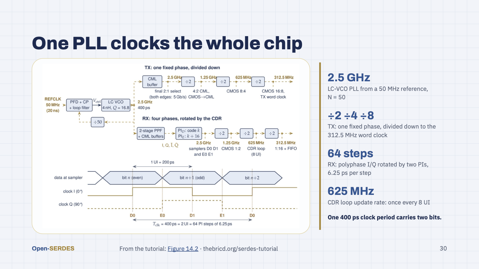
One PLL serves the whole chip. The TX divides it down with a fixed phase to the 312.5 MHz word clock. The RX makes four phases with a polyphase filter and rotates them with two phase interpolators: D0 and D1 sample the eye centers on the edges of I, E0 and E1 sample the crossings on the edges of Q. One 400 ps clock period carries two bits and spans 64 PI steps of 6.25 ps. The CDR loop updates every 8 UI, at 625 MHz. Figure 14.2 of the tutorial.
Speaker notes
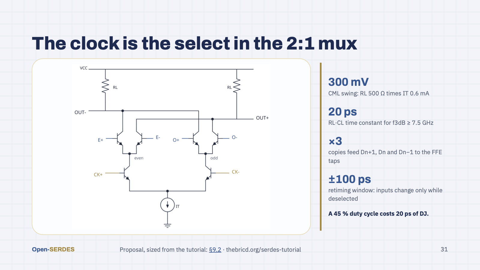
The last serializer stage needs no 5 GHz clock: the 2.5 GHz clock is the select. While CK is high the even pair drives the loads, while it is low the odd pair does, so each clock half is one 200 ps bit. HBTs switch fully with about 100 mV at the input, so a 300 mV swing on 500 Ω loads gives a gain of 5.8 where a MOS pair would give 2. The catch is duty cycle: a 45 % clock makes alternating 180 and 220 ps bits, 20 ps of deterministic jitter before the channel, so a duty-cycle corrector sits right before the mux. Built three times, it feeds D(n+1), D(n) and D(n−1) to the driver's taps. First-cut proposal; sizing from Section 9.2 of the tutorial.
Speaker notes
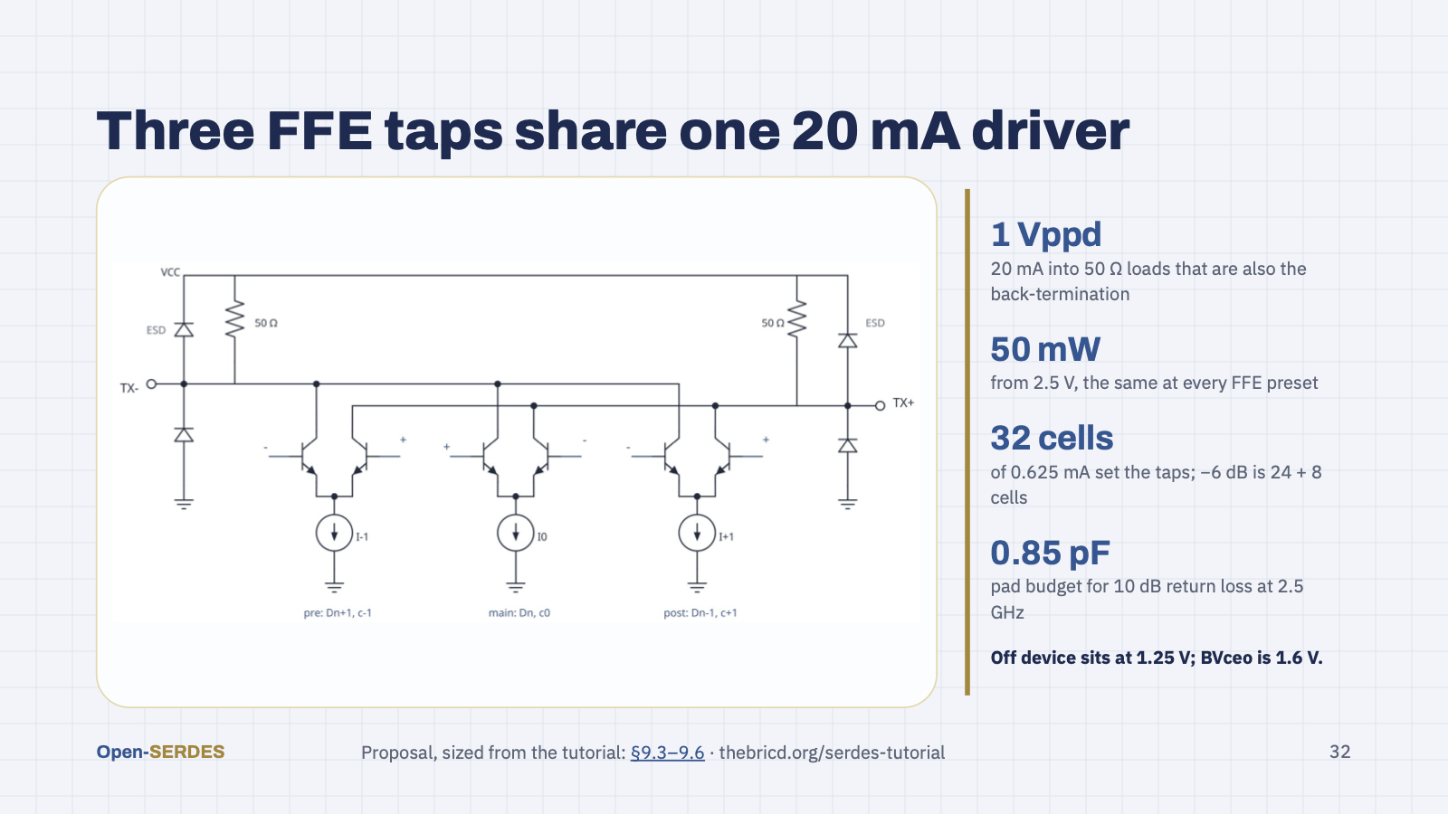
The FFE is built from current: one HBT pair per tap on the same pair of 50 Ω loads, which double as the back-termination. Each tail is a slice of one 20 mA budget, so the loads add the FIR sum and the supply current never changes with the preset. The pre and post pairs take inverted data, which makes those taps negative. 32 cells of 0.625 mA give 5-bit taps; the −6 dB preset is exactly 24 and 8 cells. Two things to check first: the off transistor sits at about 1.25 V against a BVceo of about 1.6 V, and the ESD diodes can take most of the 0.85 pF pad budget. A segmented driver or a T-coil are the upgrades, and an SST driver saves about 44 mW in a second tapeout. First-cut proposal; sizing from Sections 9.3 to 9.6 of the tutorial.
Speaker notes
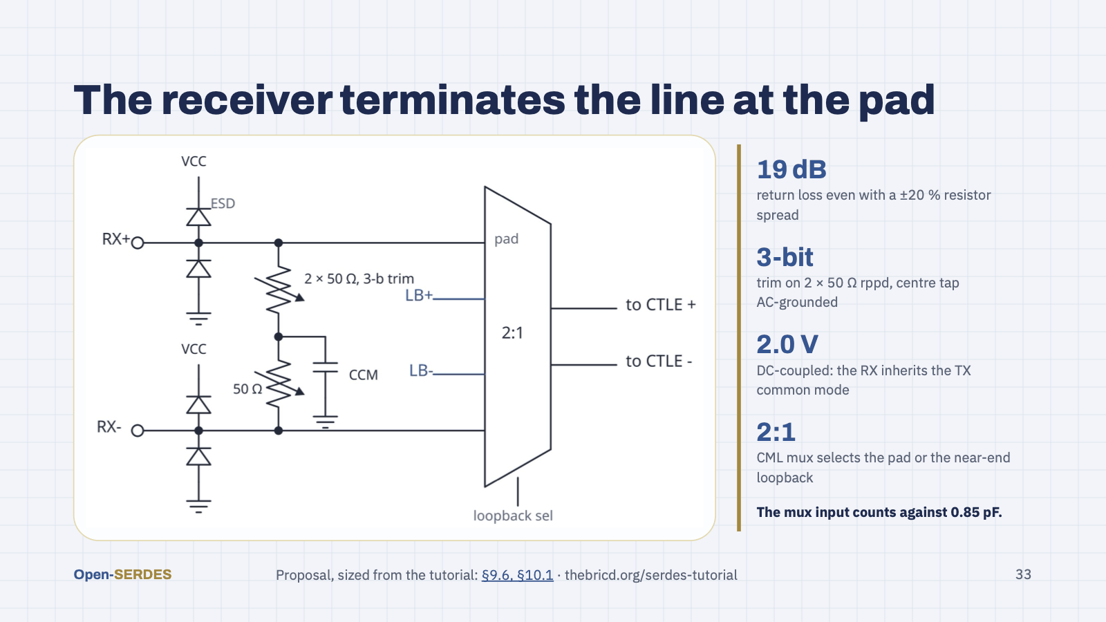
Two 50 Ω poly resistors across the pads absorb the wave, and their centre tap is AC-grounded so common-mode noise is absorbed too. Even a ±20 % resistor spread leaves 19 dB of return loss, and a 3-bit trim takes up the rest. The ESD diodes and a supply clamp sit outside the termination. The input is DC-coupled, so it inherits the 2 V common mode of the CML driver, which suits the HBT CTLE, and a CML 2:1 picks the board or the on-chip loopback from our own driver. Its input pair is part of the pad capacitance, so it counts against the 0.85 pF budget. First-cut proposal; sizing from Sections 9.6 and 10.1 of the tutorial.
Speaker notes
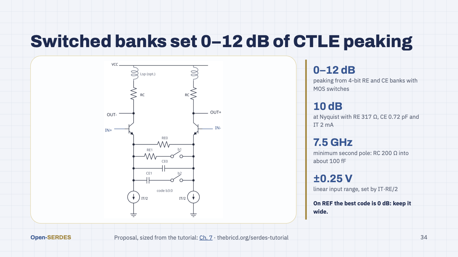
An emitter-degenerated HBT pair with two tail sources, so no bias current flows through the degeneration. Binary banks of resistors and capacitors, switched together by MOS switches, set the zero and the peaking from 0 to 12 dB; closing every resistor segment makes it a flat amplifier. With 2 mA, 317 Ω and 0.72 pF it realizes 10 dB at the 2.5 GHz Nyquist frequency. Our link model adds one point: on REF and REF-10 the best setting is 0 dB, because the FFE and DFE do the equalizing, yet the CTLE's bandwidth still costs 3.6 mV of eye. So the 0 dB code should be flat and wide, with the second pole at four times Nyquist, or have a bypass. First-cut proposal; sizing from Chapter 7 of the tutorial.
Speaker notes
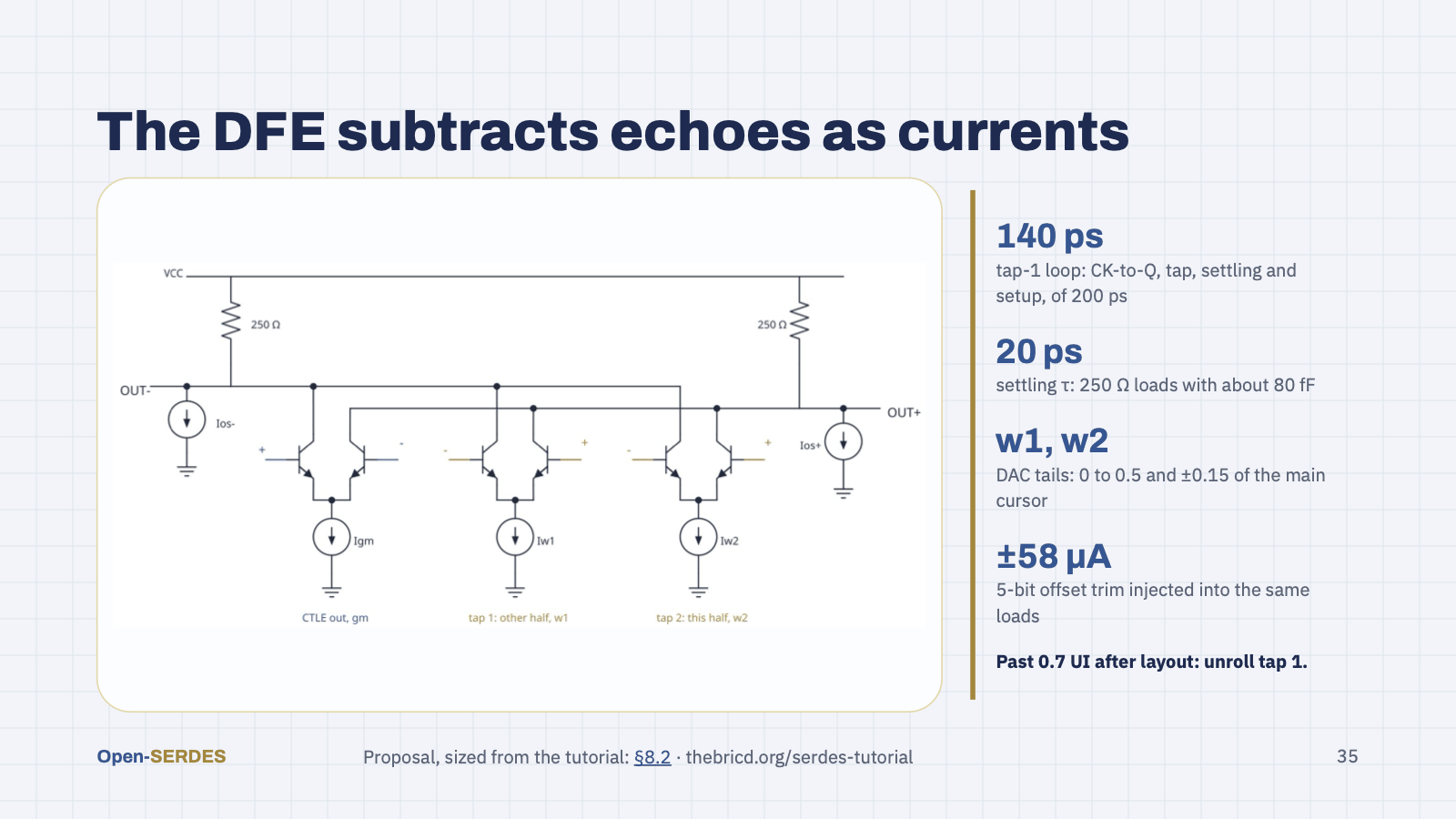
One summer per half-rate slice. The CTLE output pair and two tap pairs share 250 Ω loads; the tap-1 pair is driven by the other half's latest decision and the tap-2 pair by this half's previous one, and the decision steers each tap current to one side. DAC tails set the weights, and a 5-bit offset DAC injects a small differential current into the same loads to trim the whole path. The tap-1 loop is the critical path: clock-to-output, tap switch, 60 ps of settling and setup add up to about 140 of the 200 ps. If layout pushes it past about 0.7 UI, tap 1 is unrolled, as it is at 10 Gb/s anyway. First-cut proposal; sizing from Section 8.2 of the tutorial.
Speaker notes
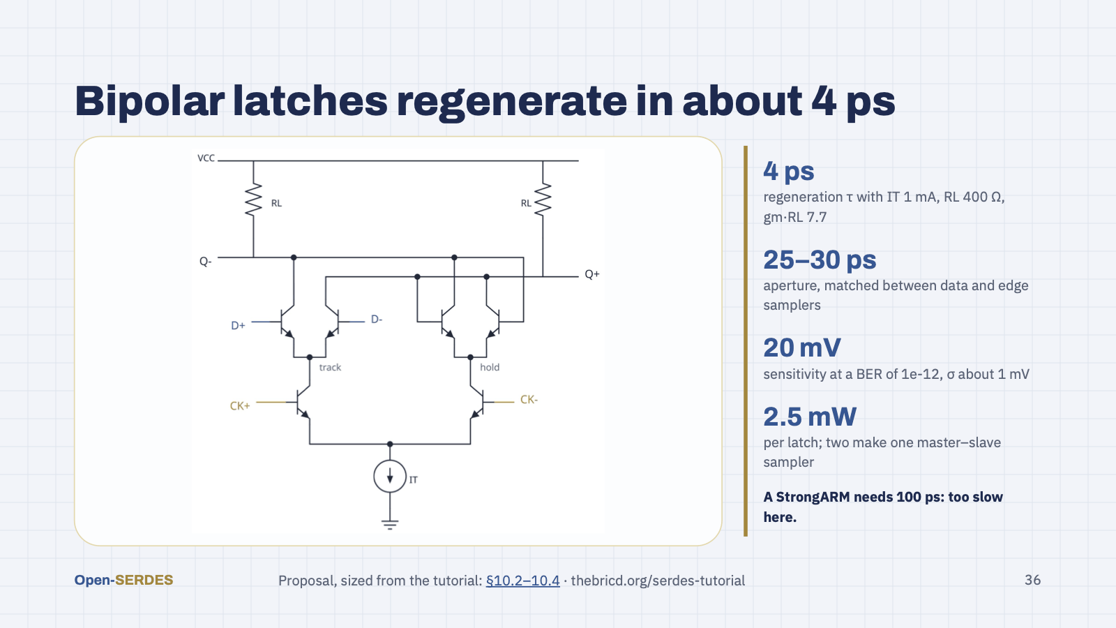
All four samplers are HBT CML master–slave flip-flops. While the clock is high the track pair follows the summer; when it falls, the cross-coupled pair holds and regenerates with a time constant of 3 to 5 ps, three to seven times faster than a CMOS StrongARM. That speed is what lets the direct-feedback DFE close its loop: the clock-to-output delay must be 25 to 35 ps. The edge samplers use the same cell so their aperture matches the data samplers; mixing latch types would make the CDR lock off-centre. Offset comes from mismatch and is trimmed through the summer, so Monte Carlo is part of the first testbench. First-cut proposal; sizing from Sections 10.2 to 10.4 of the tutorial.
Speaker notes
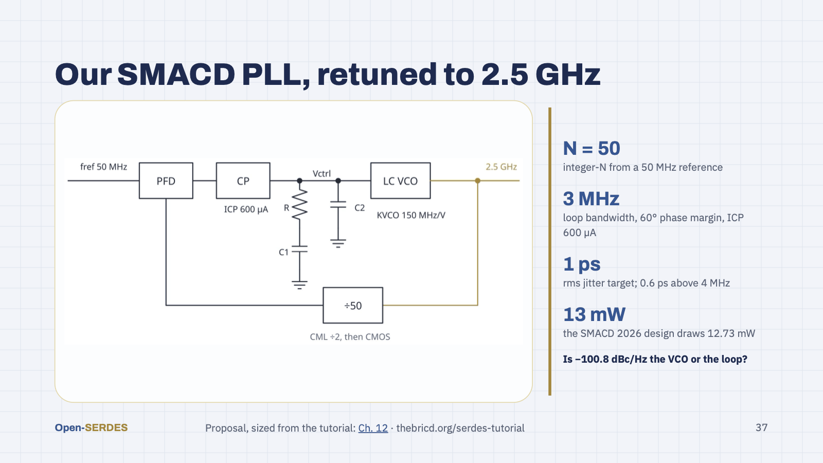
We reuse the team's SMACD 2026 PLL. Retuning it from 2.4 to 2.5 GHz is small; the bigger changes are an integer divide-by-50 in place of the fractional-N divider, a CML divide-by-2 prescaler, and a loop filter redesigned for about 3 MHz of bandwidth, where reference and VCO noise balance at about 1 ps rms. One open question matters for the jitter budget: Leeson's model predicts about −122 dBc/Hz at 1 MHz for this tank, so the measured −100.8 dBc/Hz is probably the closed loop, not the VCO. First-cut proposal; numbers from Chapter 12 of the tutorial.
Speaker notes
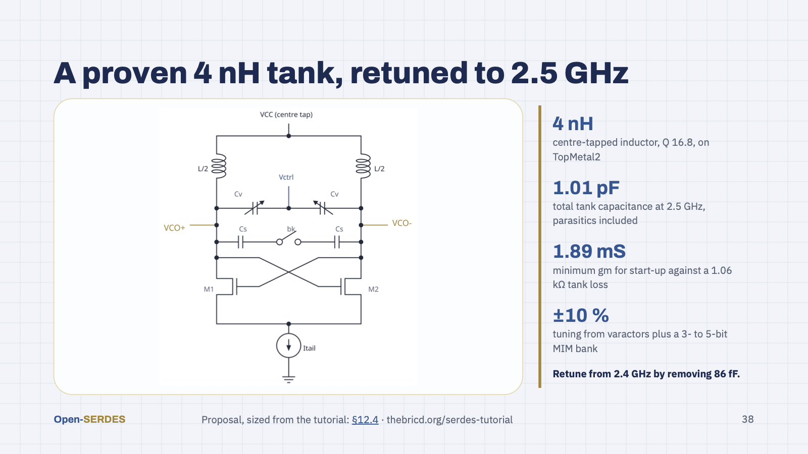
A cross-coupled LC oscillator: the pair's negative resistance cancels the tank loss, varactors set the fine tuning and the VCO gain, a switched MIM bank picks coarse bands for the corners, and the tail current sets the amplitude. We keep the proven 4 nH inductor with its Q of 16.8. At 2.5 GHz the tank needs 1.01 pF in total, 86 fF less than at 2.4 GHz, so one capacitor unit comes out. The 10 Gb/s target needs a new 10 GHz tank with a CML divide-by-2, which goes on the Phase 1 shuttle. Drawn with MOSFETs as in our design; HBTs work too with capacitive coupling. First-cut proposal; numbers from Section 12.4 of the tutorial.
Speaker notes
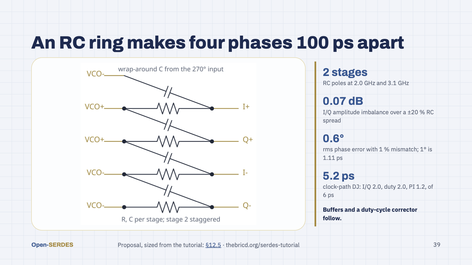
The half-rate receiver needs four clock phases exactly 100 ps apart. A polyphase filter makes them from the 2.5 GHz VCO: each output gets a resistor from its own input and a capacitor from the previous phase. One stage gives exact 90 degree steps but equal amplitude only at its pole, so a second stage with a staggered pole follows; together they hold the amplitude within 0.07 dB over process. The phase error comes from mismatch, about 0.6 degrees rms, so the last stage needs a careful common-centroid layout. Limiting CML buffers and a duty-cycle corrector restore the 5 dB the filter loses. First-cut proposal; numbers from Section 12.5 of the tutorial.
Speaker notes
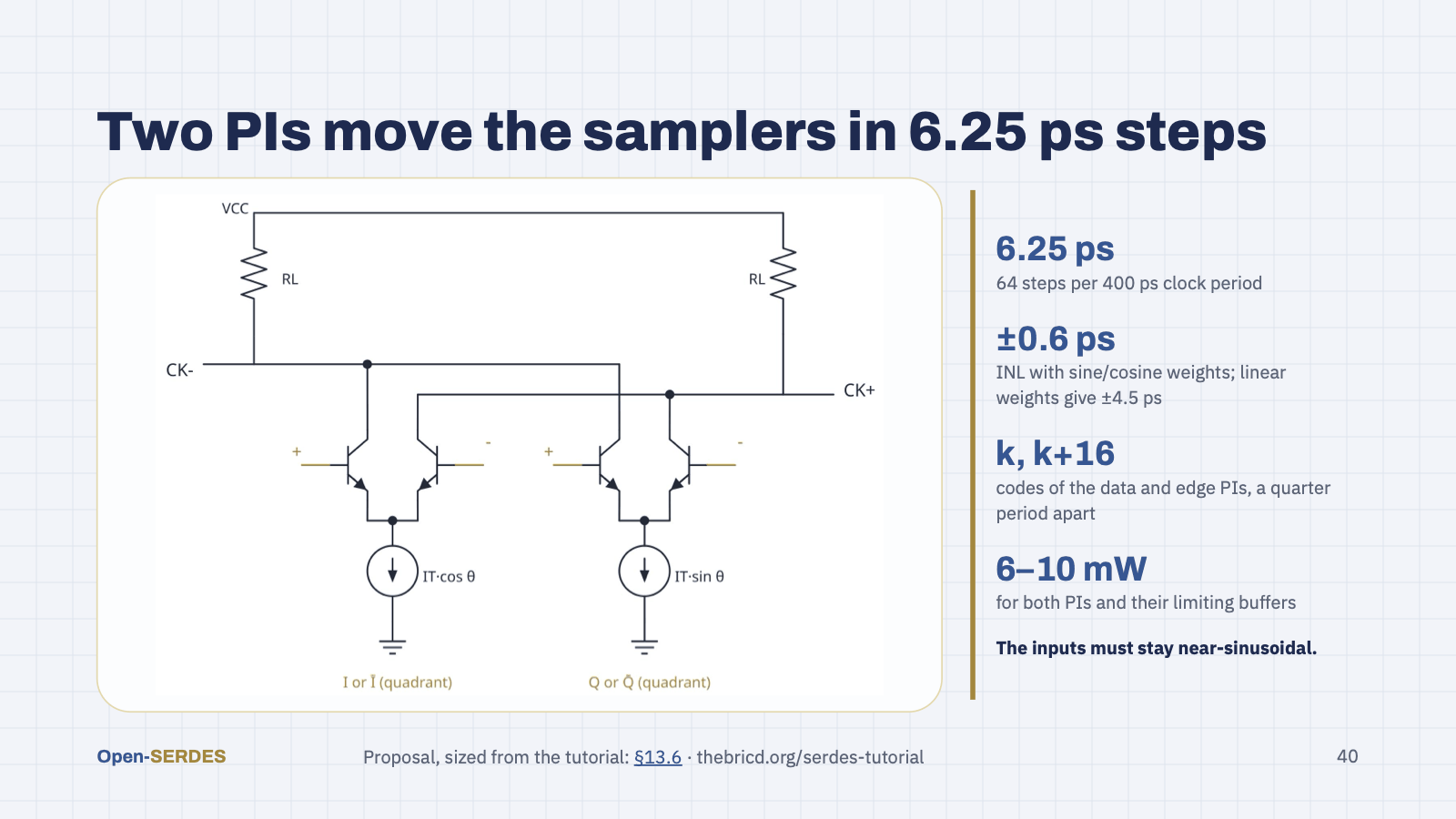
The phase interpolator adds weighted I and Q currents on shared loads. Linear weights trace the chord between the two phasors, not the arc, which gives about 4.5 ps of nonlinearity; weights taken from a quantized sine and cosine table cut it to 0.6 ps. The quadrant is chosen by swapping I and Q polarity at the inputs, and a limiting buffer removes the amplitude dip. Two copies run a quarter period apart: the data PI at code k, the edge PI at k plus 16. The CDR loop moves both every 8 UI. First-cut proposal; numbers from Section 13.6 of the tutorial.
Speaker notes
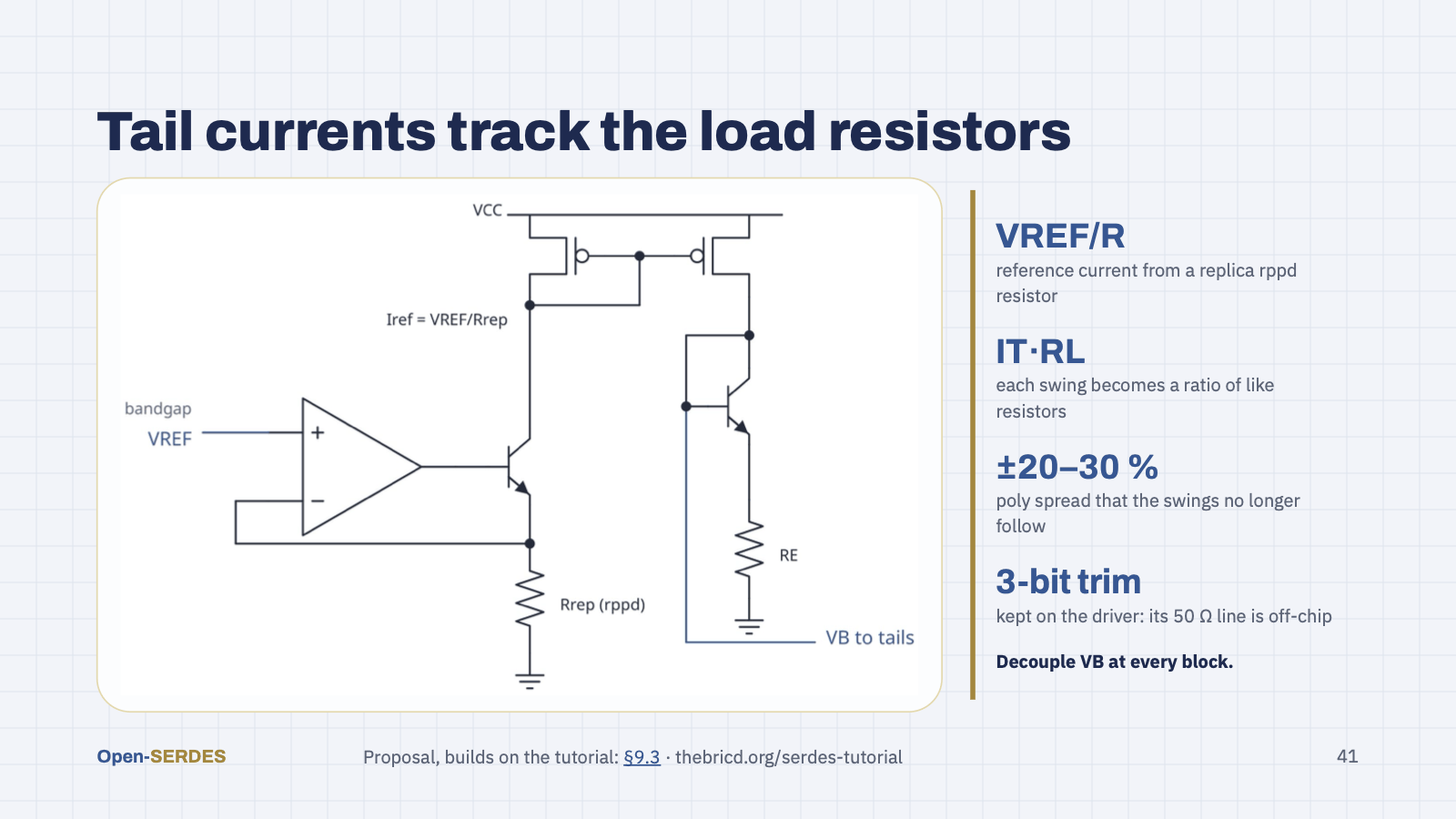
This one is our proposal rather than the tutorial's. Poly resistors spread by 20 to 30 percent, and every CML swing is a tail current times a load resistor. If an op-amp forces a bandgap voltage across a replica of the same resistor and that current biases every tail, each swing becomes a resistor ratio that only matching can disturb. Latch gain, mux swing and PI amplitude then hold across corners. The TX driver is the exception: half of its load is the 50 Ω line outside the chip, so it keeps its 3-bit termination trim. First-cut proposal; builds on Section 9.3 of the tutorial.
Speaker notes
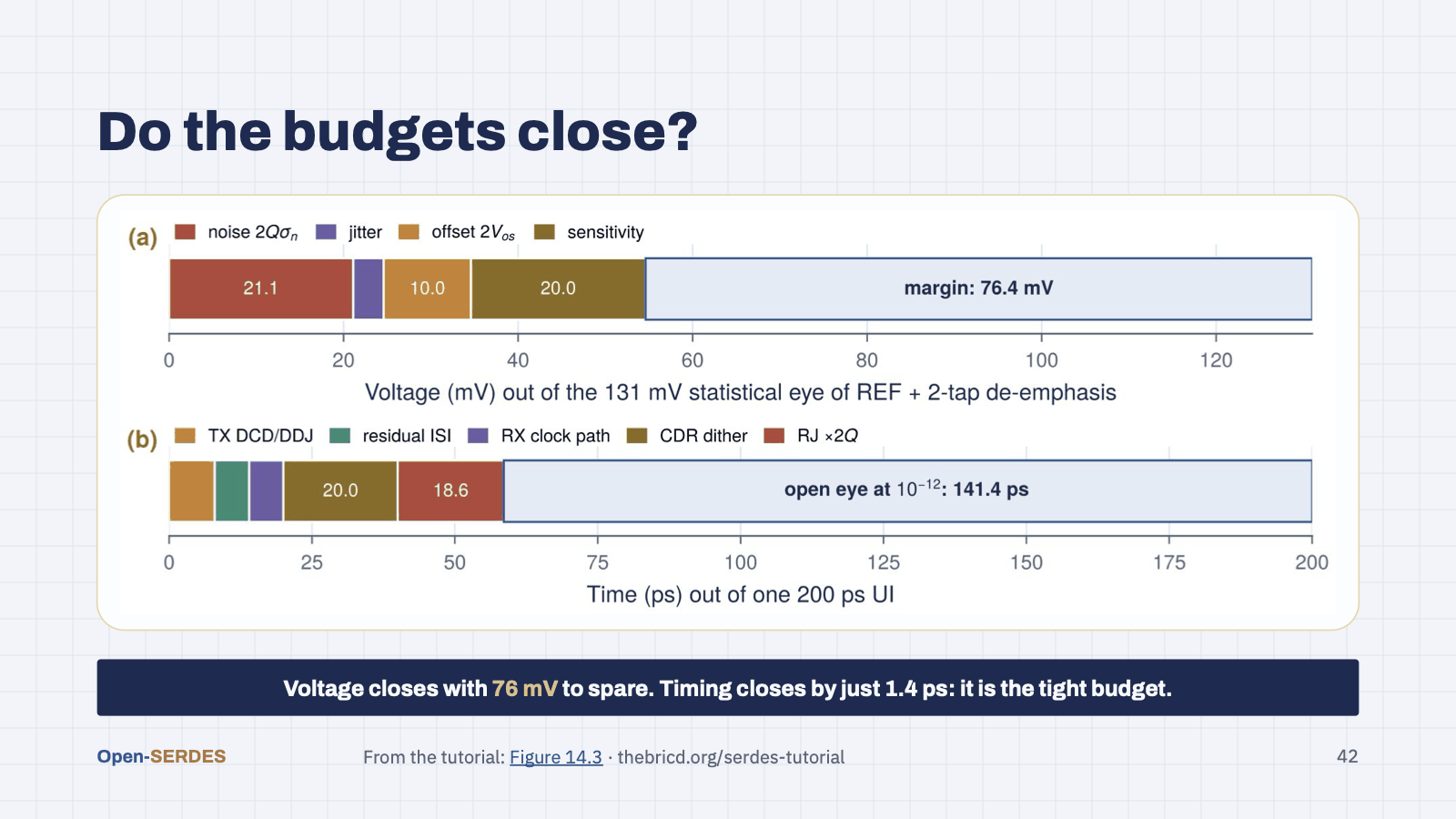
Both budgets close, but not equally. (a) Start from the 131 mV statistical eye of REF with 2-tap de-emphasis and subtract noise, jitter, offset and sampler sensitivity: 76 mV of margin remains, more than half the eye. (b) Start from one 200 ps UI and subtract the deterministic jitter linearly and 2Q times the random jitter in RSS: 141 ps remains, only 1.4 ps more than the 0.7 UI target. Clocking is where the design has the least room, and at 10 Gb/s it is the main work: the same circuits would use 0.46 UI, so every picosecond term must roughly halve. Figure 14.3 of the tutorial.
Speaker notes
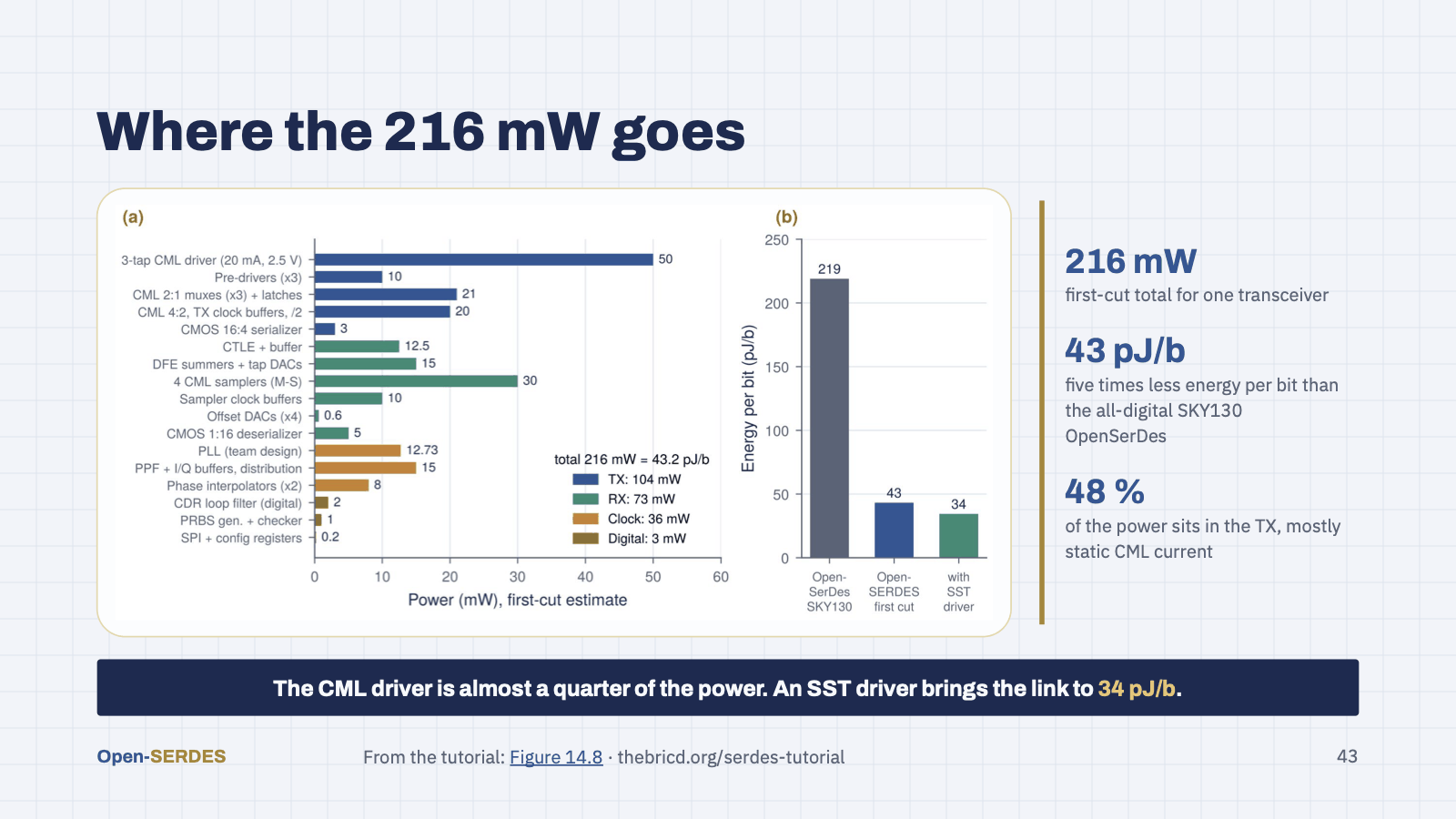
A first-cut power budget of about 216 mW, or 43 pJ/b, colored by section. The TX takes 48 percent, mostly static CML current, and the 3-tap CML driver alone is almost a quarter of the chip. The four samplers are the largest RX item, and CMOS logic is a rounding error. Right: energy per bit against the Purdue OpenSerDes in SKY130, about 219 pJ/b, and against Open-SERDES with a voltage-mode SST driver at 34 pJ/b, the first saving to go after. At 10 Gb/s the same chip draws about 280 mW, or about 28 pJ/b, because CML power hardly depends on the rate. Figure 14.8 of the tutorial.
Speaker notes
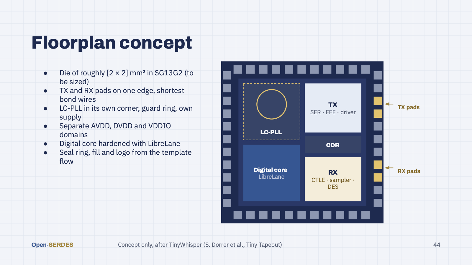
What the die could look like, in the spirit of the TinyWhisper chip render. High-speed TX and RX pads sit on one edge to keep bond wires short; the LC-PLL gets its own corner, guard ring and supply; the digital core is hardened with LibreLane. Size and placement are placeholders until the blocks exist.
Speaker notes
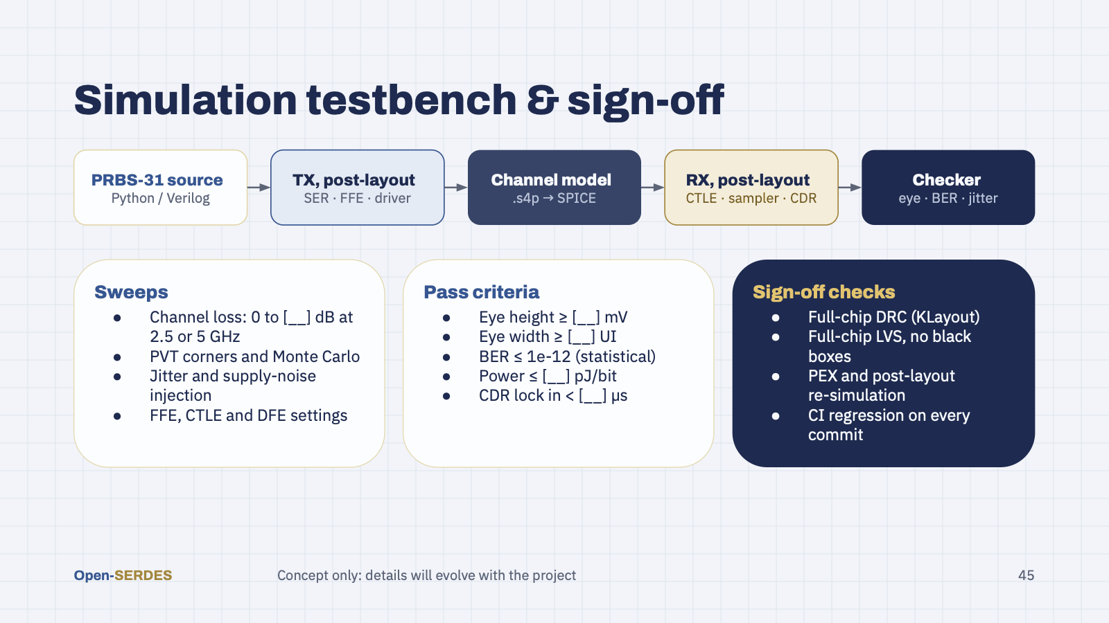
Inspired by the full top-level LVS and simulation slide. The top-level testbench drives a PRBS-31 pattern through the post-layout TX, an S-parameter channel model and the post-layout RX into a checker that reports eye, BER and jitter. We sweep channel loss, PVT, jitter and settings against pass criteria that the feasibility study will fix, and sign off with full-chip DRC and LVS without black boxes, all in CI.
Speaker notes
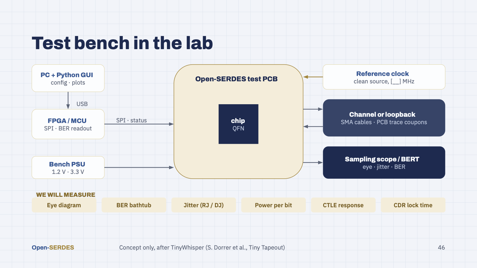
Inspired by the TinyWhisper breadboard and scope photos. A PC runs the Python GUI and talks to an FPGA or MCU board over USB; that board configures the chip over SPI and reads back the BER counter. A bench supply powers the test PCB, a clean reference clock feeds the PLL, TX goes out through SMA into a channel or loopback and back into RX, and a sampling scope or BERT captures eyes, jitter and BER.
Speaker notes
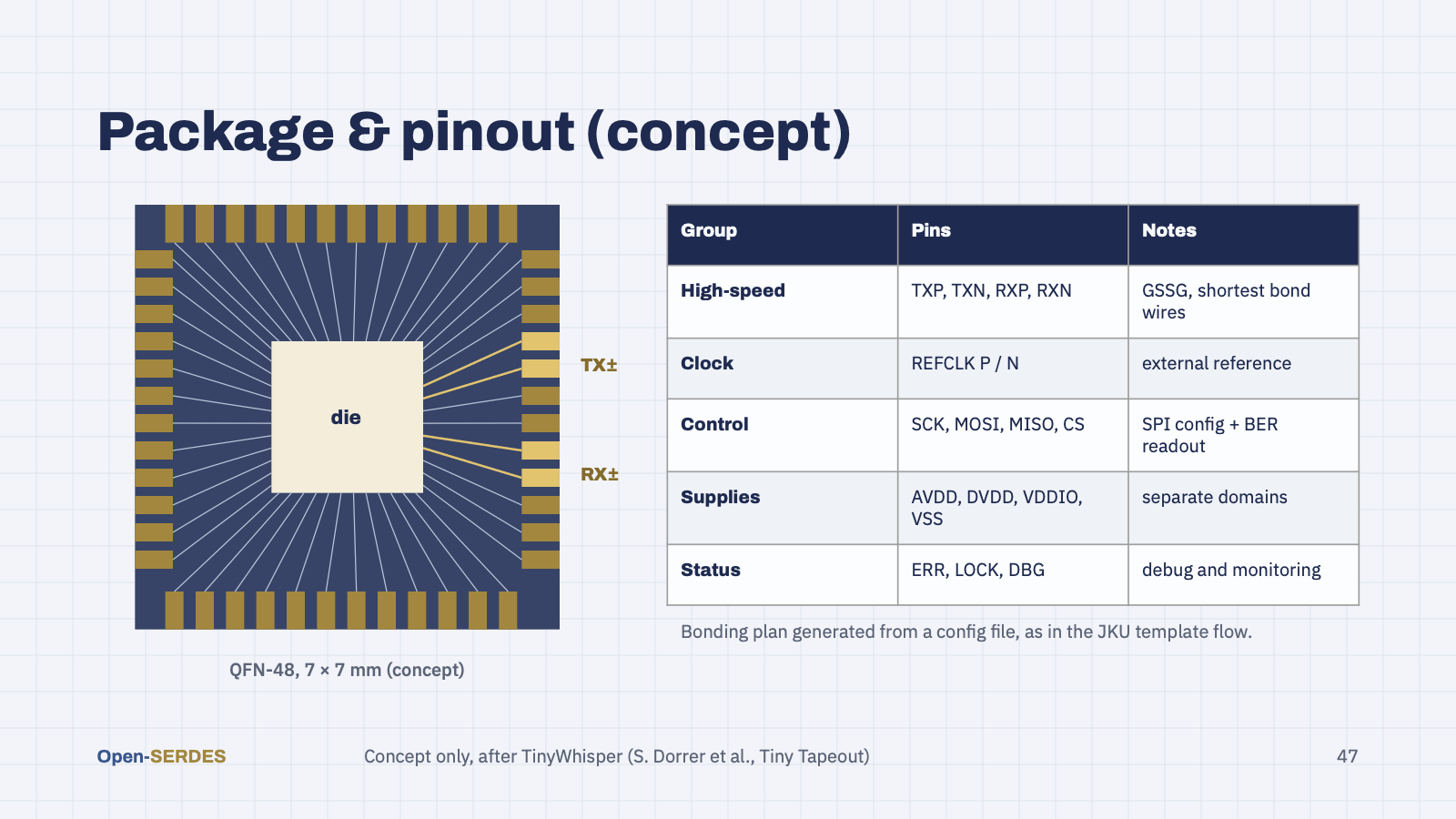
Inspired by the TinyWhisper bonding diagram. A QFN package with the high-speed TX and RX pins on one side and the shortest bond wires, an external reference clock, SPI for configuration and BER readout, separate supply domains, and a few status pins. As in the JKU template, the bonding plan would be generated from a config file.
Speaker notes
Part 5: how we get there, and where you come in.
Speaker notes
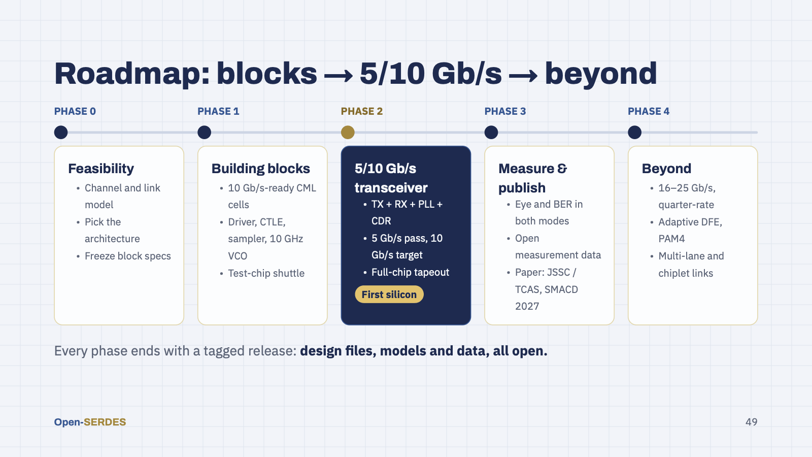
Five phases. Phase 0 is the feasibility study: an industry-standard channel, the link model, the architecture decision and frozen block specs. Phase 1 builds the building blocks, sized for 10 Gb/s, and tapes them out on a test shuttle such as Tiny Tapeout IHP or an IHP open MPW, together with the new 10 GHz VCO. Phase 2 is the headline goal: a complete transceiver with TX, RX, PLL and CDR and a rate select, verified with an on-chip PRBS loopback and taped out as a full chip. Its pass criterion is 5 Gb/s over the 1 m reference channel; 10 Gb/s over half that channel is the design target. Phase 3 is measurement in both modes and publication, with open data, targeting IEEE JSSC or TCAS and SMACD 2027. Phase 4 goes beyond: 16 to 25 Gb/s with a quarter-rate datapath, adaptive DFE, PAM4 for lossy channels, multiple lanes and chiplet-style links. [Add dates once the timeline is agreed.]
Speaker notes
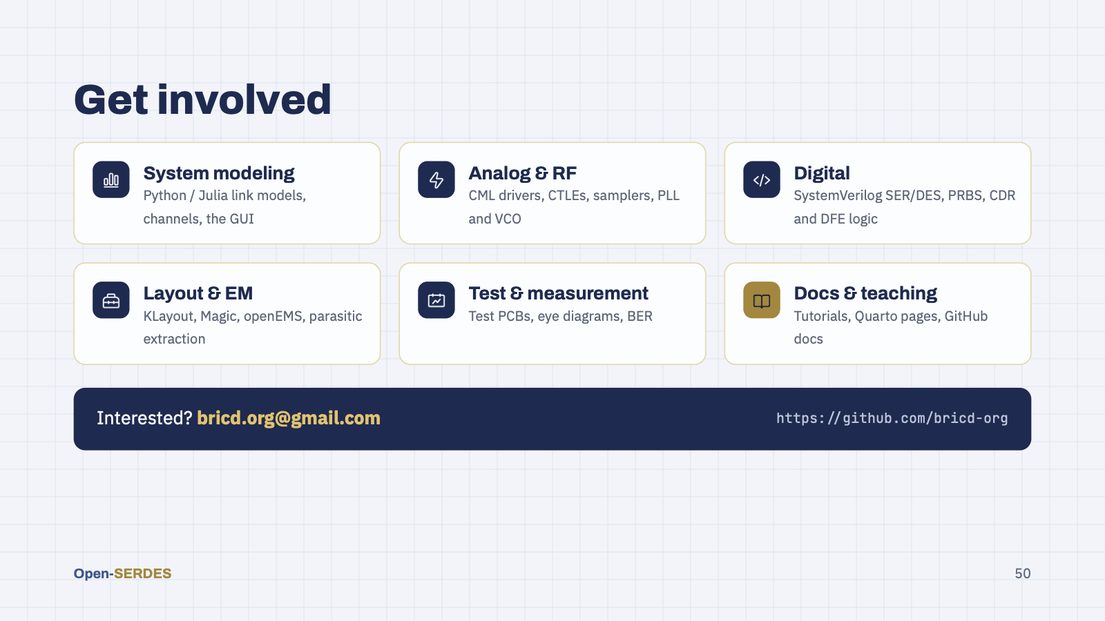
We need people across the whole stack, and you do not need to know everything to start: curiosity and willingness to learn count most. System modellers in Python or Julia; analog and RF designers for CML, CTLE, samplers and the PLL; digital designers for the serializer, deserializer, PRBS and CDR logic; layout and EM people; anyone with a lab bench for measurement; and people who love writing tutorials. Everything will live publicly on GitHub.
Speaker notes
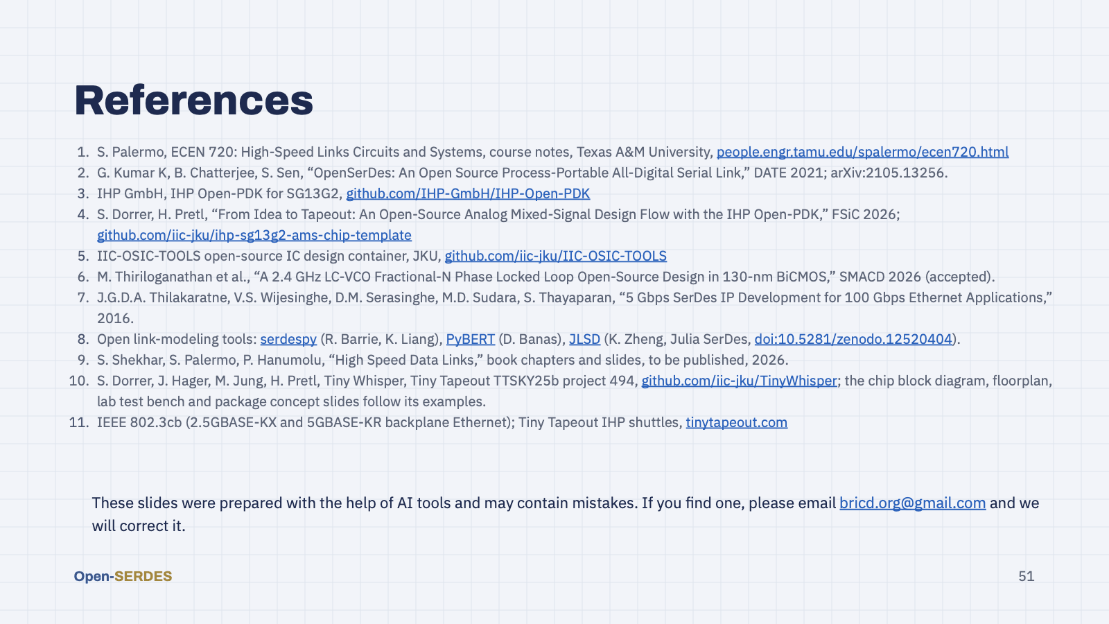
Reference slide; leave it up during questions if useful.