Chapter 10Receiver Front-End and Samplers
The receiver must turn a 100 mV, 200 ps-wide eye into clean logic levels, \(10^{12}\) times in a row without a mistake. This chapter builds the circuits that do it.
In this chapter you will learn
Draw the Open-SERDES receiver from pad to 16-bit word, and set its termination, common mode and coupling.
List what a sampler must deliver (sensitivity, offset, aperture, metastability, kick-back, noise) and derive the regeneration time constant of the StrongARM and the HBT CML latch.
Compute the metastability error probability and explain why edge samplers need extra latch stages.
Estimate sampler offset from Pelgrom’s law and size a 5-bit calibration DAC.
Build a circuit-level noise and sensitivity budget that supports the system budget of Section 4.4.
Deserialize half-rate decisions to 16 bits at 312.5 MHz and cross into the core clock domain.
10.1The receiver front-end
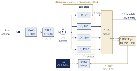
Figure 10.1 shows the receive path. The 100 Ω termination absorbs the wave at the pad. The CTLE (Section 7.4) boosts the high frequencies, and the DFE summer subtracts the post-cursor echoes of earlier decisions (Section 8.2). Four samplers then decide. At half rate, \(D_0\) and \(D_1\) sample the data at 0° and 180° of the 2.5 GHz clock, one bit each per clock period. \(E_0\) and \(E_1\) sample the transitions between them at 90° and 270°. The deserializer turns these four 2.5 Gb/s streams into 16 data bits and 16 edge bits at 312.5 MHz. The CDR logic uses both to steer the phase interpolator (Chapter 13), which shifts the four clock phases until \(E_0\) and \(E_1\) sit on the zero crossings.
Termination and common mode
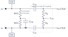
The RX termination is two 50 Ω poly resistors in series across the inputs, with their center tap AC-grounded by a capacitor \(C_\mathrm{CM}\) (Figure 10.2). Differential signals see 100 Ω. Common-mode noise sees a low impedance and is absorbed too. The termination sits right at the pad, inside the ESD diodes, and shares the pad capacitance budget of Section 9.6. The CTLE input pair needs its own common mode, and the input stage must stay linear for the largest signal: long runs on a short channel arrive at nearly the full \(\pm0.5\,\mathrm{V}\). A switchable input attenuator, or the CTLE’s own gain control, handles short channels (Section 7.4).
DC or AC coupling
With DC coupling the RX inherits the TX common mode: about 2.0 V from the CML driver of Section 9.4, which suits an HBT CTLE on the same 2.5 V supply. AC coupling with series capacitors lets each side set its own common mode, at the price of a high-pass corner. A run of \(N\) identical bits then droops by \(1-e^{-NT_\mathrm{b}/\tau}\) (baseline wander). Off-chip 100 nF capacitors in the 100 Ω loop give \(\tau=10\,\mu\mathrm{s}\), and PRBS31’s 31-bit run droops by only 0.06 %. On chip, 2 pF into a 10 kΩ bias resistor gives \(\tau=20\,\mathrm{ns}\) and a 27 % droop, which needs DC-balanced (scrambled or 8b/10b) data. Open-SERDES is DC-coupled for near-end loopback and has board footprints for off-chip capacitors.
10.2Samplers
A sampler (clocked comparator, or slicer) looks at its input at one instant and amplifies the sign of the difference to a full logic level. It is a positive-feedback latch, and everything we want from it follows from that. For Open-SERDES it must deliver:
Sensitivity: a correct decision at \(10^{-12}\) for inputs down to about 20 mVpp, the value budgeted in Section 4.4;
Offset below about 5 mV after calibration (Section 10.4);
Aperture well below 1 UI, so that it samples a point rather than averaging the eye, and a sampling bandwidth well above \(f_\mathrm{N}\);
Regeneration fast enough that even tiny inputs resolve in time (Section 10.3), and a clock-to-output delay that fits the DFE loop of Section 8.2;
Low kick-back: the large internal swings must not couple back into the CTLE and disturb the other three samplers;
Low noise: at least the \(kT/C\) noise of its internal nodes, \(\sqrt{kT/C}=0.45\,\mathrm{mV}\) at 20 fF.
10.2.1The StrongARM latch
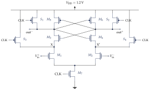
The StrongARM latch (Figure 10.3) is the standard CMOS comparator [29, 30]. It draws no static current and produces rail-to-rail outputs. Its operation has four phases:
Reset (CLK low): \(S_1\)–\(S_4\) precharge out\(^\pm\), X and X\('\) to \(V_\mathrm{DD}\), and \(M_7\) is off.
Integration (CLK rises): \(M_7\) turns on. The input pair \(M_1/M_2\) discharges X and X\('\), then the output nodes, with currents \(I_D\pm g_\mathrm{m}\,v_\mathrm{in}/2\). The common mode falls and a differential voltage grows linearly.
Regeneration: when the outputs have fallen by \(\lvert V_\mathrm{TP}\rvert\), the PMOS \(M_5/M_6\) turn on. The two cross-coupled inverters (\(M_3/M_5\), \(M_4/M_6\)) now amplify the difference exponentially. The input pair is in triode and no longer sees the input.
Decision: one output returns to \(V_\mathrm{DD}\) and the other falls to ground. An SR latch holds the result while the next reset begins [31].
Regeneration time constant
In regeneration each inverter, biased near its switching point, is a transconductance \(g_\mathrm{m}\) (NMOS plus PMOS) driving its own output capacitance \(C\) from the other output: \(C\,\dot v_1=-g_\mathrm{m}v_2\) and \(C\,\dot v_2=-g_\mathrm{m}v_1\). Subtracting, the difference \(\Delta V=v_1-v_2\) obeys \(C\,\dot{\Delta V}=g_\mathrm{m}\Delta V\), a growing exponential. The integration phase sets its starting value: the outputs fall at \(I_D/C\), so regeneration begins after \(t_1=C\lvert V_\mathrm{TP}\rvert/I_D\), and by then the input pair has built \(\Delta V(t_1)=g_\mathrm{m,in}v_\mathrm{in}t_1/C=A_\mathrm{int}\,v_\mathrm{in}\).
Key equation · StrongARM regeneration and decision time
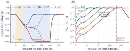
\[\Delta V(t)=A_\mathrm{int}\,v_\mathrm{in}\,e^{(t-t_1)/\tau},\qquad \tau=\frac{C}{g_\mathrm{m}},\qquad t_\mathrm{dec}=t_1+\tau\ln\frac{V_L}{A_\mathrm{int}\,v_\mathrm{in}} . \tag{10.1}\] Each factor of 10 less input adds \(\tau\ln10=2.3\tau\) to the decision time. \(V_L\) is the swing the next stage needs.
Figure 10.4 shows a behavioral model with the numbers of Worked Example 10.1: \(C=20\,\mathrm{fF}\), \(I_D=200\,\mu\mathrm{A}\) and \(\lvert V_\mathrm{TP}\rvert=0.4\) V give \(t_1=40\,\mathrm{ps}\) and \(A_\mathrm{int}=3\); the cross-coupled pair gives \(\tau=20\,\mathrm{fF}/1.5\,\mathrm{mS}\approx13\,\mathrm{ps}\). A 1 mV input decides in 109 ps, a 10 V input in 169 ps.
10.2.2The HBT CML latch
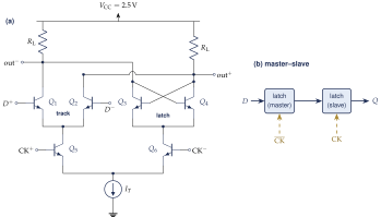
The CML latch (Figure 10.5) is the bipolar alternative [24]. While CK is high, the track pair \(Q_1/Q_2\) is an ordinary CML buffer and the outputs follow the input with time constant \(R_\mathrm{L}C\). When CK falls, the tail current switches to the cross-coupled pair \(Q_3/Q_4\), which holds and amplifies whatever difference the outputs carried at that instant. Two latches on opposite clock phases form a master–slave flip-flop.
Key equation · CML latch regeneration
\[C\,\dot{\Delta V}=\Big(g_\mathrm{m}-\frac{1}{R_\mathrm{L}}\Big)\Delta V\qquad\Longrightarrow\qquad \tau=\frac{R_\mathrm{L}C}{g_\mathrm{m}R_\mathrm{L}-1},\qquad g_\mathrm{m}=\frac{I_T/2}{V_T}. \tag{10.2}\] The cross-coupled pair adds \(g_\mathrm{m}\Delta V\) of current and the loads remove \(\Delta V/R_\mathrm{L}\); regeneration needs a loop gain \(g_\mathrm{m}R_\mathrm{L}>1\).
Why it is fast in SG13G2
With \(I_T=1\,\mathrm{mA}\), each side carries 0.5 mA and \(g_\mathrm{m}=19.3\,\mathrm{mS}\); \(R_\mathrm{L}=400\,\Omega\) gives a 400 mV swing and \(g_\mathrm{m}R_\mathrm{L}=7.7\). With \(C=30\,\mathrm{fF}\), Equation (10.2) gives \(\tau=1.8\,\mathrm{ps}\), and 3–5 ps once base resistance and \(C_\mu\) are included. That is three to seven times faster than the StrongARM, because the HBT’s \(g_\mathrm{m}/I=1/V_T\) and its 300 GHz \(f_T\) give large \(g_\mathrm{m}\) with little capacitance. The latch also kicks back less, since its current never changes, and its sampling instant does not move with the input common mode. Its cost is static power: 2.5 mW per latch from 2.5 V.
The Open-SERDES choice
All four samplers are HBT CML master–slave flip-flops. The data samplers must, because the direct-feedback DFE needs a clock-to-output delay of 25–35 ps (Section 8.2); a 1.2 V StrongARM with its SR latch needs 100 ps or more for small inputs. The edge samplers use the same circuit so that data and edge samplers have the same aperture delay, as the next paragraph shows. A StrongARM remains the right choice where a decision can wait, such as the DFE’s error sampler (Section 8.3) or slow monitors.
Aperture
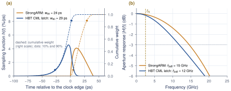
A real sampler does not take an instantaneous sample. Its output is a weighted average \(\int v_\mathrm{in}(t)h(t)\,dt\) with \(\int h=1\), where \(h(t)\) is the sampling function [32]. The aperture \(w_{80}\) is the time that holds the central 80 % of the weight. Its Fourier transform is the sampler’s own bandwidth. Figure 10.6 compares the two latches. The StrongARM integrates during the 40 ps after the clock edge; the CML latch remembers the input with its track time constant \(R_\mathrm{L}C=12\,\mathrm{ps}\) before the edge. Both apertures are about 25–30 ps (0.12–0.14 UI), and both bandwidths, 12–15 GHz, cost less than 0.2 dB at \(f_\mathrm{N}\). But their centroids differ by 23 ps. A StrongARM edge sampler next to CML data samplers would make the CDR lock 0.12 UI away from the true eye center. Keep \(w_{80}\le0.2\) UI with sharp clock edges, and use one sampler type for data and edge.
10.3Metastability
If the input is close enough to zero, the latch has not reached a valid logic level \(V_L\) when its time \(T\) runs out. It is then metastable, and downstream logic may read it either way, or both ways at once. By Equation (10.1) the latch fails only if its starting value is below \(V_Le^{-T/\tau}\), that is, if \(\lvert v_\mathrm{in}\rvert<V_Le^{-T/\tau}/A\), where \(A\) is the gain in front of the regenerative node.
Key equation · Metastability error probability
\[P_\mathrm{meta}=\frac{2V_L}{A\,\Delta V}\,e^{-T/\tau},\qquad\text{and for cascaded stages}\quad P_\mathrm{meta}\propto e^{-(T_1/\tau_1+T_2/\tau_2+\dots)} . \tag{10.3}\] The input is assumed spread uniformly over a range \(\Delta V\); the fraction that lands in the failing window of width \(2V_Le^{-T/\tau}/A\) is \(P_\mathrm{meta}\). Each latch stage behind the first multiplies the probability by its own \(e^{-T/\tau}\).
Worked Example 10.1 · StrongARM metastability, data versus edge samplers
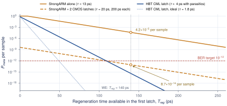
Timing: the half-rate clock period is 400 ps, so evaluation lasts 200 ps. Integration takes \(t_1=40\,\mathrm{ps}\) and the SR latch needs about 20 ps, which leaves \(T=140\,\mathrm{ps}\) of regeneration with \(\tau=13\,\mathrm{ps}\): a gain of \(e^{10.8}=4.8\times10^4\).
Data sampler: reaching \(V_L=0.6\,\mathrm{V}\) needs \(0.6/4.8\times10^4=12\,\mu\mathrm{V}\) at the latch, or 4 µV at the input with \(A_\mathrm{int}=3\). An equalized eye never puts the data sample that close to zero, so data samplers are safe.
Edge sampler: it samples the zero crossing on purpose, so its input is often tiny. Take the input spread over \(\pm100\,\mathrm{mV}\) (\(\Delta V=0.2\,\mathrm{V}\)) and \(A=3\): \(P_\mathrm{meta}=(2\cdot0.6/0.6)\,e^{-10.8}=\mathbf{4.2\times10^{-5}}\) per sample, or \(10^5\) undefined decisions per second at 2.5 GS/s. That is far too many for a digital CDR loop.
Fix: two more latch stages, each with 200 ps and \(\tau\approx20\,\mathrm{ps}\), multiply by \(e^{-20}\): \(P_\mathrm{meta}=\mathbf{8.7\times10^{-14}}\), below the BER target. A metastable edge decision then costs one bang-bang vote, which the loop filter averages away.
HBT CML latch: with \(\tau\approx4\,\mathrm{ps}\) and the same 140 ps, \(P_\mathrm{meta}\approx4\times10^{-16}\) in the master latch alone (with \(V_L=0.2\,\mathrm{V}\)).
Edge samplers need extra stages
A data sampler sees an open eye; an edge sampler is aimed at the zero crossing, so it is metastable thousands of times more often. Always put at least two more latch stages between an edge sampler and the CDR logic, and count their regeneration time. In Open-SERDES the CML slave latch and the first CMOS flip-flops of the deserializer provide them.
10.4Offset and calibration
Two transistors drawn identically are not identical. Random dopant and edge fluctuations give the threshold voltages of a matched pair a random difference whose standard deviation falls with gate area [33]. A sampler with mismatched input devices therefore has an input-referred offset \(V_\mathrm{os}\): it decides as if its threshold were \(V_\mathrm{os}\) instead of zero.
Key equation · Pelgrom mismatch and calibration sizing
\[\sigma_{V_\mathrm{os}}\approx\frac{A_{VT}}{\sqrt{WL}},\qquad \text{range}=\pm3\sigma_{V_\mathrm{os}},\qquad \mathrm{LSB}=\frac{6\sigma_{V_\mathrm{os}}}{2^n},\qquad \lvert V_\mathrm{os,res}\rvert\le\frac{\mathrm{LSB}}{2}. \tag{10.4}\] Halving \(\sigma\) needs four times the area, and so four times the input capacitance. A DAC is cheaper.
Worked Example 10.2 · Sizing the offset DAC
Given: an input pair of \(W/L=4\,\mu\mathrm{m}/0.13\,\mu\mathrm{m}\) (\(WL=0.52\,\mu\mathrm{m}^{2}\)) and \(A_{VT}\approx3.5\,\mathrm{mV}\,\mu\mathrm{m}\). That \(A_{VT}\) is an assumption for 130 nm; extract the real value by Monte Carlo if the SG13G2 models include mismatch.
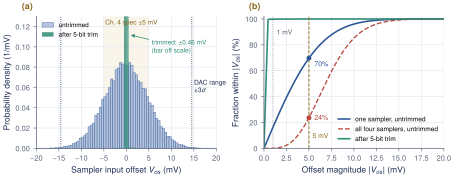
Offset: \(\sigma=3.5/\sqrt{0.52}=4.9\,\mathrm{mV}\), so \(\pm3\sigma=\pm14.6\,\mathrm{mV}\). Untrimmed, only 70 % of samplers meet \(\lvert V_\mathrm{os}\rvert<5\,\mathrm{mV}\), and all four in one receiver do so on only 24 % of chips (Figure 10.8).
DAC: a residual of \(\pm1\,\mathrm{mV}\) needs \(\mathrm{LSB}\le2\,\mathrm{mV}\), so \(n\ge\log_2(29.2/2)=3.9\). Choose 5 bits: LSB = 0.91 mV, residual \(\pm0.46\,\mathrm{mV}\). After trim, 99.8 % of samplers are within 1 mV.
The no-calibration alternative needs \(\sigma=1\,\mathrm{mV}\), or \(WL=12.2\,\mu\mathrm{m}^{2}\): 24 times the area, with the capacitance, kick-back and slower \(\tau\) that come with it.
Calibrating the Open-SERDES receiver
The HBT pairs of the CML samplers match better than MOS pairs, but the CTLE, the summer and the load resistors add offsets of their own. Open-SERDES therefore trims the whole path, one DAC per sampler, by injecting a differential current into the DFE summer load (Figure 10.9). The total current stays constant, so the common mode does not move. Referred to the input with unity front-end gain, one LSB of 0.91 mV across the 250 Ω summer load is 3.6 µA, and the full \(\pm16\) LSB range is \(\pm58\,\mu\mathrm{A}\). The procedure is a short digital loop: short the inputs to the common mode, count ones and zeros for a few thousand cycles, step the code toward 50/50, repeat until it toggles by one LSB, then freeze it. Capacitive trim on the StrongARM’s internal nodes is the alternative for CMOS samplers; it costs aperture time.

What this means for your design
Do not buy offset with area. Use minimum-capacitance input devices for speed, calibrate the whole path with a 5-bit DAC sized for \(\pm3\sigma\), and leave the 5 mV of the system budget for drift between calibrations. Simulate offset with Monte Carlo mismatch, never with ideal devices.
10.5Noise and the sensitivity budget
Section 4.4 budgeted the receiver with three numbers: \(\sigma_\mathrm{n}=1.5\,\mathrm{mV}\) rms input-referred noise, \(V_\mathrm{os}=5\,\mathrm{mV}\) after calibration, and a sampler sensitivity \(V_\mathrm{sens}=20\,\mathrm{mV}\). Here we check them against the circuits. The sensitivity of a sampler collects its own Gaussian noise \(\sigma_s\) at the BER multiplier, the minimum overdrive \(V_\mathrm{min}\) that resolves in time (metastability, hysteresis and kick-back memory), and its residual offset [24]:
Key equation · Sampler sensitivity
\[V_\mathrm{sens}\approx 2Q\,\sigma_s+V_\mathrm{min}+2\lvert V_\mathrm{os,res}\rvert,\qquad 2Q=14.07\ \text{at}\ 10^{-12}. \tag{10.5}\]
Worked Example 10.3 · Circuit-level noise and sensitivity budget
All terms are rms and referred to the RX input, conservatively with unity front-end gain.
| Source | \(\sigma\) (mV) | How it was estimated |
|---|---|---|
| Termination and line, 50 Ω diff. | 0.10 | 0.91 nV/\(\sqrt{\mathrm{Hz}}\) over an 11.8 GHz noise bandwidth |
| CTLE (shot noise, \(R_E\), \(R_C\)) | 0.25 | Section 7.4 densities; confirm with .noise |
| DFE summer loads | 0.32 | \(\sqrt{2kT/C}\), \(C=80\,\mathrm{fF}\) |
| Sampler, input-referred | 1.0 | \(kT/C\) floor 0.45–0.64 mV; 0.7–0.85 mV measured [32] |
| Total (RSS) | 1.08 | system budget assumes 1.5 |
Sensitivity: with \(\sigma_s=1\,\mathrm{mV}\), \(V_\mathrm{min}\approx5\,\mathrm{mV}\) and the 5-bit residual of 0.46 mV, Equation (10.5) gives \(14.1+5+0.9=\mathbf{20}\) mV, the value of Section 4.4.
Margin: with the circuit noise, the linear budget of Section 4.4 becomes \(131-14.07\times1.08-3.5-10-20=\mathbf{82}\) mV instead of 76 mV. Since \(V_\mathrm{sens}\) already contains the sampler’s own noise and residual offset, the system budget counts them twice and is about 15 mV conservative.
The budget follows Palermo’s rule for noise sources [24]: classify each one as bounded or Gaussian, and as proportional to swing or independent of it. Thermal noise, offset and sensitivity are independent of swing, so they shrink in relative terms as the eye grows. Residual ISI and crosstalk are proportional to swing, and no TX amplitude can beat them. With 82 mV of margin, the receiver circuits are not the weak link; equalization is.
10.6The deserializer
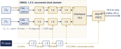
The first 1:2 of the deserializer is free: a half-rate receiver already delivers even and odd bits on separate samplers. The rest mirrors the transmitter (Figure 10.10). Each sampler’s 2.5 Gb/s output is converted from CML to CMOS levels and enters a 1:8 tree of CMOS 1:2 stages clocked at 1.25 GHz, 625 MHz and 312.5 MHz. That is 400 ps per bit at the first CMOS flip-flop, or 9.5 FO4, which a 1.2 V CMOS flip-flop handles; a CMOS 1:2 demux is also far less sensitive to duty cycle than the TX mux. The two data lanes interleave into the 16-bit word, and the two edge lanes give 16 edge bits for the CDR logic. The clocks come from the recovered 2.5 GHz clock through \(\div2\) stages, so the whole tree lives in the recovered clock domain.
Crossing into the core clock
The recovered 312.5 MHz clock and the core’s 312.5 MHz clock, which comes from the local PLL, have the same frequency in near-end loopback, or when both ends share a reference, but an unknown and wandering phase. A small asynchronous FIFO, 4–8 words deep with Gray-coded pointers, absorbs that. If the far end has its own reference (\(\pm100\,\mathrm{ppm}\) each), the frequencies differ by up to 200 ppm: one word slips every 5000 words, or every 16 µs. That needs an elastic buffer with skip and insert symbols, which is a protocol feature. For bring-up, run the PRBS checker directly in the recovered domain, before the FIFO, so a BER measurement needs no clock crossing at all.
10.7RX design checklist
Table 10.1 collects the RX checks and a first-cut power estimate of about 70 mW, without the PLL, phase interpolator and CDR logic (Section 14.6).
| Block | Check before layout | Power |
|---|---|---|
| Termination, ESD, pad | 100 Ω diff., AC-grounded center tap; \(C_p<0.85\) pF; RL \(\ge10\) dB at \(f_\mathrm{N}\) | – |
| CTLE and buffer | linear range for the long-run level; 0–12 dB peaking (2 mA + 3 mA) | 12.5 mW |
| DFE summers (\(\times2\)), taps | settles within the tap-1 budget; offset DAC injection (6 mA) | 15 mW |
| 4 CML samplers (M–S) | \(\tau\le5\) ps; \(t_\mathrm{CK\to Q}\le35\) ps; same type for data and edge (12 mA) | 30 mW |
| I/Q clock buffers | sharp edges (\(w_{80}\le0.2\) UI); phase error \(\le5^{\circ}\) (5.6 ps) | 10 mW |
| Offset DACs (\(\times4\)) | 5 bits, \(\pm3\sigma\) range, LSB 0.91 mV | 0.6 mW |
| Deserializer (1.2 V) | two extra latch stages behind \(E_0\)/\(E_1\); FIFO or in-domain PRBS checker | 5 mW |
| Total RX | 27 mA from 2.5 V, 4 mA from 1.2 V | \(\approx\)73 mW |
Key takeaways
The Open-SERDES receiver is termination, CTLE, DFE summer and four half-rate samplers (data at 0°/180°, edges at 90°/270°), followed by a 1:16 deserializer and the CDR logic.
A latch amplifies exponentially, \(\Delta V\propto e^{t/\tau}\): \(\tau=C/g_\mathrm{m}\approx13\) ps for a 130 nm StrongARM and \(\tau=R_\mathrm{L}C/(g_\mathrm{m}R_\mathrm{L}-1)\approx\) 2–5 ps for an SG13G2 HBT CML latch.
Open-SERDES uses HBT CML master–slave samplers everywhere: the DFE loop needs their 25–35 ps clock-to-output, and one sampler type keeps the data and edge apertures aligned.
\(P_\mathrm{meta}=(2V_L/A\Delta V)\,e^{-T/\tau}\). A lone StrongARM edge sampler gives \(4\times10^{-5}\); two extra latch stages bring it below \(10^{-13}\).
Pelgrom’s law gives \(\sigma\approx4.9\,\mathrm{mV}\) for a small 130 nm pair; a 5-bit DAC over \(\pm3\sigma\) leaves \(\pm0.46\) mV.
The circuit noise is about 1.1 mV rms and the sensitivity about 20 mV, which supports the system budget with about 80 mV of margin.
Half rate gives the first 1:2 for free; CMOS does the rest, and a small FIFO crosses from the recovered to the core clock.
Generated from book/tutorial/chapters/10_rx.tex. Figure, table and equation numbers match the PDF edition.