Chapter 2Signals, Systems and the Language of Links
Five ideas carry the whole book: the unit interval, the pulse response, the cursors, the eye diagram and the bit-error rate.
In this chapter you will learn
describe an NRZ stream by its unit interval, bit rate and Nyquist frequency, and explain why most of its energy lies below \(f_\mathrm{N}\);
generate PRBS test patterns with an LFSR and know what PRBS7 and PRBS31 stress;
predict how a simple low-pass channel slows edges, using impulse, step and frequency responses;
build a received waveform from shifted pulse responses and read the main, pre- and post-cursors;
read an eye diagram (height, width, crossing, slope) and turn an eye opening and an rms noise into a BER.
Here the channel is deliberately simple, a one-pole RC filter or a short line; the realistic REF channel waits for Section 3.7, and the tools carry over unchanged. This chapter is standard background, covered in more depth in Palermo’s ECEN 720 lectures [4, 13] and in Dally and Poulton [14].
2.1NRZ signaling: bits, symbols and the unit interval
A link carries bits \(b_k \in \{0,1\}\). The simplest way to put them on a wire is non-return-to-zero (NRZ) signaling, also called PAM2: each bit becomes a symbol \(a_k = 2b_k - 1 \in \{-1,+1\}\), and the transmitter holds the voltage \(A\,a_k\) for one bit period (Figure 2.1). In Open-SERDES, \(A = 0.5\,\mathrm{V}\) (1 Vppd). One symbol lasts one unit interval (UI). NRZ sends one bit per symbol, so the bit rate \(f_\mathrm{b}\) equals the baud rate; PAM4 sends two (Section 4.5).
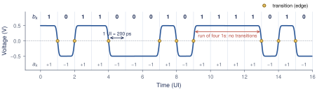
The fastest NRZ pattern, 1010…, is a square wave with a period of \(2T_\mathrm{b}\). Its fundamental frequency is the Nyquist frequency, the single most important frequency in link design.
Key equation · Unit interval and Nyquist frequency
\[T_\mathrm{b}= 1\,\mathrm{UI}= \frac{1}{f_\mathrm{b}}, \qquad f_\mathrm{N}= \frac{1}{2T_\mathrm{b}} = \frac{f_\mathrm{b}}{2} \tag{2.1}\] For Open-SERDES: \(f_\mathrm{b}= 5\,\mathrm{Gb}/\mathrm{s}\), \(T_\mathrm{b}= 200\,\mathrm{ps}\) and \(f_\mathrm{N}= 2.5\,\mathrm{GHz}\).
The spectrum of random NRZ
An NRZ waveform is a sum of rectangular pulses, \[x(t) = A\sum_n a_n\, g(t - nT_\mathrm{b}),\] where \(g(t)\) is a 1-UI rectangle with Fourier transform \(G(f) = T_\mathrm{b}\,\mathrm{sinc}(fT_\mathrm{b})\,e^{-j\pi fT_\mathrm{b}}\) and \(\mathrm{sinc}(u) = \sin(\pi u)/(\pi u)\). If the symbols are independent and equally likely to be \(\pm1\), then \(\mathrm{E}[a_n a_m]\) is 1 for \(n = m\) and 0 otherwise. The cross terms average away, and each pulse contributes its own energy spectrum \(A^2\lvert G(f)\rvert^2\) once every \(T_\mathrm{b}\) seconds. The power spectral density (PSD) is therefore \(A^2\lvert G(f)\rvert^2/T_\mathrm{b}\):
Key equation · PSD of random NRZ
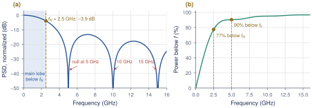
\[S_x(f) = A^2\,T_\mathrm{b}\,\mathrm{sinc}^2(fT_\mathrm{b}), \qquad \text{nulls at } f = f_\mathrm{b}, 2f_\mathrm{b}, \dots \tag{2.2}\]
Figure 2.2a plots Equation (2.2). The main lobe runs from DC to the first null at \(f_\mathrm{b}= 5\,\mathrm{GHz}\), and at \(f_\mathrm{N}\) the PSD is \(\mathrm{sinc}^2(0.5) = (2/\pi)^2\), or −3.9 dB. Integrating the PSD (Figure 2.2b) shows that 77% of the power lies below \(f_\mathrm{N}\) and 90% below \(f_\mathrm{b}\).
Worked Example 2.1 · Where the power of a 5 Gb/s stream sits
The fraction of power below \(f_\mathrm{N}\) is \(2\int_0^{1/2}\mathrm{sinc}^2(u)\,du = 0.774\), so an ideal low-pass filter at 2.5 GHz would still pass three quarters of the power. The REF channel’s 17.4 dB at 2.5 GHz, a factor of 7.4 in amplitude, attacks exactly that band.
What this means for your design
Treat \(f_\mathrm{N}= 2.5\,\mathrm{GHz}\) as the frequency your link lives at: quote channel loss there, and give every block enough bandwidth around it (Section 2.5). The energy above \(f_\mathrm{b}\) is under 10% and mostly edge sharpness.
2.2PRBS test patterns
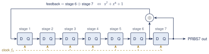
Testing needs data that looks random but is reproducible, so the receiver can check every bit. A pseudo-random bit sequence (PRBS) does this. It comes from a linear-feedback shift register (LFSR): a chain of \(n\) flip-flops whose input is the XOR of two of its outputs. Figure 2.3 shows PRBS7, defined by the polynomial \(x^7 + x^6 + 1\): the new bit is stage 6 XOR stage 7. With the right taps, the register steps through all \(2^n - 1\) non-zero states before it repeats, producing a maximal-length sequence.
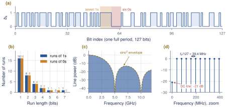
A PRBS-\(n\) sequence has a few properties worth remembering (Figure 2.4):
Period \(2^n - 1\) bits, during which every \(n\)-bit word except all zeros appears exactly once.
Nearly balanced: \(2^{n-1}\) ones and \(2^{n-1} - 1\) zeros (64 and 63 for PRBS7).
Run lengths: the longest run is \(n\) ones and \(n-1\) zeros. Half of all runs have length 1, a quarter length 2, and so on, like a fair coin.
Line spectrum: because the pattern repeats, its spectrum is a set of lines spaced \(f_\mathrm{b}/(2^n-1)\) apart under the same \(\mathrm{sinc}^2\) envelope as random NRZ.
Choosing a PRBS
PRBS7 repeats every 25.4 ns and never holds a level longer than 7 UI: ideal for bring-up. PRBS31 (\(x^{31}+x^{28}+1\)) has runs of up to 31 bits and a period of 0.43 s; its low-frequency content stresses AC coupling (baseline wander), long ISI tails and the CDR’s ability to hold phase without transitions, so it is the compliance pattern. Model work uses PRBS13 (8191 bits), far longer than the channel’s ISI memory. Real protocols also encode the data: 8b/10b (PCIe 1/2, USB 3.2 Gen 1, SATA) maps each byte to 10 bits with at most five equal bits in a row and long-term DC balance, at 25% overhead.
A short pattern can hide a long problem
If the link remembers more bits than the pattern varies over, the eye looks too good: PRBS7 can pass where PRBS31 fails on baseline wander or a long reflection. Confirm designs with a pattern longer than every memory in the link.
2.3Linear systems in one section
Between the TX output and the RX sampler, the link is close to a linear time-invariant (LTI) system, fully described by its impulse response \(h(t)\), the output for a very short unit-area pulse. For any input \(x(t)\) the output is the convolution \[y(t) = (x * h)(t) = \int_{-\infty}^{\infty} x(\tau)\,h(t-\tau)\,d\tau , \qquad Y(f) = X(f)\,H(f), \tag{2.3}\] where the frequency response \(H(f)\) is the Fourier transform of \(h(t)\). Convolution becomes multiplication, so cascaded blocks multiply. Gains are quoted in decibels, \(\lvert H\rvert_\mathrm{dB} = 20\log_{10}\lvert H(f)\rvert\): −3 dB is a factor 0.707, −6 dB one half, −20 dB one tenth, and in a cascade the dB values add. A Bode plot shows \(\lvert H\rvert_\mathrm{dB}\) against log frequency.
The one-pole system
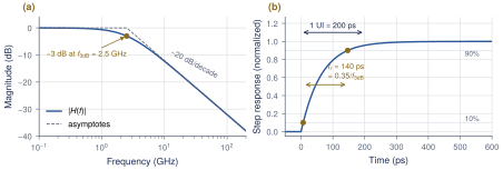
A resistor driving a capacitor is the simplest low-pass filter and a good first model of a slow channel or a CML stage with load \(R_\mathrm{L}C_\mathrm{L}\) (Figure 2.5):
Key equation · One-pole low-pass filter
\[H(f) = \frac{1}{1 + jf/f_\mathrm{3dB}},\quad h(t) = \frac{1}{\tau}e^{-t/\tau},\quad s(t) = 1 - e^{-t/\tau},\quad t_r^{10\text{--}90} = \tau\ln 9 \approx \frac{0.35}{f_\mathrm{3dB}} \tag{2.4}\]
Here \(\tau = RC = 1/(2\pi f_\mathrm{3dB})\), \(s(t)\) is the unit step response (for \(t \ge 0\)) and \(t_r\) is the 10–90% rise time. Above \(f_\mathrm{3dB}\) the gain falls by 20 dB per decade.
Worked Example 2.2 · What bandwidth keeps ISI small at 5 Gb/s?
For a bit to barely affect the next, the output must almost settle within one UI. One UI after a step, a one-pole system still has an error of \(e^{-T_\mathrm{b}/\tau}\). Asking for at most 5%:
\(e^{-T_\mathrm{b}/\tau} \le 0.05 \;\Rightarrow\; T_\mathrm{b}/\tau \ge \ln 20 = 3.0 \;\Rightarrow\; \tau \le 66.8\,\mathrm{ps}\);
\(f_\mathrm{3dB} = 1/(2\pi\tau) \ge 3.0/(2\pi\times200\,\mathrm{ps}) = 2.38\,\mathrm{GHz}\);
the rise time is then \(0.35/2.38\,\mathrm{GHz} = 147\,\mathrm{ps} \approx 0.73\,\mathrm{UI}\).
A one-pole bandwidth close to the Nyquist frequency, \(f_\mathrm{3dB} \approx f_\mathrm{N}= 2.5\,\mathrm{GHz}\), keeps the ISI to a few percent. Section 2.5 turns this into an exact eye opening.
2.4The pulse response
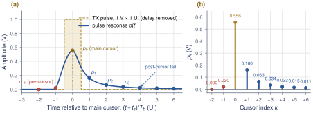
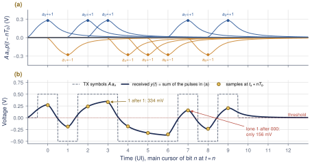
A link never sends impulses; it sends 1-UI rectangles. The response to one isolated rectangle of 1 V and width \(T_\mathrm{b}\) is the pulse response \(p(t)\), the most useful single picture of a link: \[p(t) = h(t) * \Pi_{T_\mathrm{b}}(t) = \int_{t-T_\mathrm{b}}^{t} h(\tau)\,d\tau = s(t) - s(t - T_\mathrm{b}), \tag{2.5}\] where \(\Pi_{T_\mathrm{b}}(t)\) is 1 for \(0 \le t < T_\mathrm{b}\): a step up, then a step down one UI later. An NRZ waveform is a sum of shifted, signed rectangles and the channel is linear, so the received signal is a sum of shifted, signed pulse responses (Figure 2.7). Sample it once per UI at \(t_\mathrm{s}+ nT_\mathrm{b}\), with \(t_\mathrm{s}\) usually at the peak of \(p(t)\). The samples of the pulse response at integer UI offsets are the cursors \(p_{k} = p(t_\mathrm{s}+ kT_\mathrm{b})\) (Figure 2.6). The main cursor \(p_{0}\) carries the wanted bit. Post-cursors \(p_{k}\), \(k > 0\), are the tail of a pulse sent \(k\) bits earlier. Pre-cursors \(p_{k}\), \(k < 0\), are the leading edge of a pulse sent \(\lvert k\rvert\) bits later.
Key equation · Superposition of pulse responses
\[y(t) = A\sum_n a_n\, p(t - nT_\mathrm{b}) \qquad\Longrightarrow\qquad y_n = y(t_\mathrm{s}+ nT_\mathrm{b}) = \underbrace{A\,a_n\,p_{0}}_{\text{wanted}} \;+\; \underbrace{A\sum_{k\neq0} a_{n-k}\,p_{k}}_{\text{intersymbol interference (ISI)}} \tag{2.6}\]
The channel acts like an FIR filter whose taps are the cursors; everything except the main cursor is intersymbol interference (ISI), the echo of neighboring bits at the sampling instant.
Worked Example 2.3 · Reading a sample from the cursors
Bit 7 in Figure 2.7 is a lone 1 after three 0s, followed by a 0. With \(A = 0.5\,\mathrm{V}\) and the cursors of Figure 2.6:
wanted signal: \(Ap_{0} = 0.5\times0.5561 = 278\,\mathrm{mV}\);
the three previous 0s and the next 0 subtract: \(-A(p_{1}+p_{2}+p_{3}+p_{-1}) = -0.5\,(0.1605+0.0629+0.0340+0.0205) = -139\,\mathrm{mV}\);
the older bits (\(a_3 = a_2 = a_0 = +1\), \(a_1 = -1\)) add \(0.5\,(0.0216+0.0151-0.0112+0.0087) = 17\,\mathrm{mV}\).
The sample is \(278 - 139 + 17 = 156\,\mathrm{mV}\), as simulated: ISI took 44% of the wanted signal.
What this means for your design
The cursors are the channel’s fingerprint, and every equalizer in Part II acts on them: the TX FFE reshapes the pulse (Chapter 6), the CTLE sharpens it (Chapter 7) and the DFE subtracts post-cursors (Chapter 8). Faced with a new channel, plot its pulse response first.
Lab 1: pulse response and cursors
lab1_channel.py turns the REF channel’s \(S_{21}\) into a pulse response and its cursors. Lengthen the line and watch \(p_{1}/p_{0}\) grow (Section 16.2).
2.5ISI: how pulse spreading closes the eye
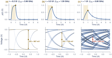
The one-pole channel shows in closed form how bandwidth turns into ISI. Its pulse response peaks at the end of the bit, \(t = T_\mathrm{b}\). Sampling there and writing \(r = e^{-T_\mathrm{b}/\tau}\) gives \(p_{0} = 1 - r\) and \(p_{k} = (1-r)\,r^{k}\) for \(k \ge 1\), with no pre-cursors. The post-cursors form a geometric series that sums to \(r\). The worst case for a 1 is that every earlier bit is a 0, so each tail pulls it down. The smallest 1 is then \(A(p_{0} - \sum_{k\ge1}p_{k})\), and by symmetry the eye opening at the sampling instant is
Key equation · Worst-case eye of a one-pole channel
\[\mathrm{EH} = 2A\Bigl(p_{0} - \sum_{k\ge1}p_{k}\Bigr) = 2A\,\bigl(1 - 2e^{-T_\mathrm{b}/\tau}\bigr), \qquad \frac{T_\mathrm{b}}{\tau} = 2\pi f_\mathrm{3dB}T_\mathrm{b}= \pi\,\frac{f_\mathrm{3dB}}{f_\mathrm{N}} \tag{2.7}\]
Figure 2.8 shows the pulse and the eye for three time constants. With \(\tau = 0.2\,\mathrm{UI}\) (\(f_\mathrm{3dB} = 4.0\,\mathrm{GHz}\)) the eye is 98.7% open. At \(\tau = 0.5\,\mathrm{UI}\) (1.6 GHz) it is 73% open, and at \(\tau = 1\,\mathrm{UI}\) (0.8 GHz) only 26%. The eye closes completely when \(r = 1/2\), that is \(\tau = T_\mathrm{b}/\ln 2 = 1.44\,\mathrm{UI}\), or \(f_\mathrm{3dB} = 552\,\mathrm{MHz}\). For the bandwidth of Worked Example 2.2, \(f_\mathrm{3dB} = f_\mathrm{N}\), the exponent is \(\pi\) and \(\mathrm{EH} = 2A(1 - 2e^{-\pi}) = 0.91 \times 2A\).
Subtracting the magnitudes of all other cursors from the main cursor works for any channel; this is peak-distortion analysis (Section 4.2). For the 10 dB line of Figure 2.6 it gives 230 mV out of 1 V; for the REF channel it is negative: the eye is closed.
Design rule of thumb
Each one-pole block in the data path needs \(f_\mathrm{3dB} \gtrsim f_\mathrm{N}= 2.5\,\mathrm{GHz}\) to cost less than about 10% of eye height. A cascade of several poles has less bandwidth than any single one, so in practice each CML stage of Open-SERDES should reach 0.7–1 \(f_\mathrm{b}\) (3.5–5 GHz).
2.6Eye diagrams
An eye diagram cuts the received waveform into 2-UI windows aligned to the bit clock and overlays them (Figure 2.9). Every bit pattern draws its own trace, so the overlay shows at a glance how much the patterns differ at each instant.
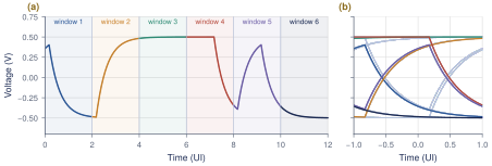
Figure 2.10 names the parts you will measure throughout this book.
Eye height (EH): the vertical opening at the sampling instant, between the lowest 1 and the highest 0. It must beat noise, offset and sampler sensitivity.
Eye width (EW): the horizontal opening at the threshold, between adjacent crossings. It must beat clock jitter and the sampler aperture.
Crossing points: where edges cross the threshold. Their spread in time is jitter; their mean is what the CDR locks to.
Optimal sampling point: the instant and threshold with the most margin both ways.
Slope near the crossing: it converts timing error into voltage error, \(\Delta v \approx (dV/dt)\,\Delta t\).
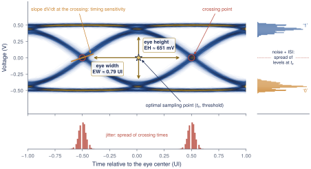
With the slope of Figure 2.10, sampling 4 ps off near an edge costs about \(2.8 \times 4 \approx 11\,\mathrm{mV}\). Noise eats the eye vertically and jitter horizontally; the next section asks how much is tolerable.
An eye is only as deep as the number of bits behind it
A simulated eye of \(10^4\) bits only shows events more frequent than about \(10^{-4}\); a \(7\sigma\) noise peak will almost never appear. An open eye in a short simulation says nothing about \(10^{-12}\). Section 4.3 computes the eye at that probability directly.
Lab 2: PRBS7 eye through the REF channel
lab2_prbs_eye.py draws the PRBS7 eye before and after the REF channel. The output eye is closed (\(-78\,\mathrm{mV}\)): the motivation for Part II (Section 16.3).
2.7Noise and the bit-error rate
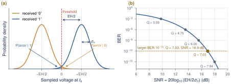
The receiver compares each sample \(y_n\) with a threshold at 0, and an error happens when noise pushes a sample across it. With a worst-case eye of height EH, a 1 arrives at least \(\mathrm{EH}/2\) above the threshold and a 0 at least \(\mathrm{EH}/2\) below it. Add Gaussian noise \(n \sim \mathcal{N}(0, \sigma_\mathrm{n}^2)\) from the termination, the front end and the sampler (Figure 2.11a). A 1 is read as a 0 when \(n < -\mathrm{EH}/2\): \[\begin{align} P(\text{error}\mid 1) &= \int_{-\infty}^{-\mathrm{EH}/2} \frac{1}{\sqrt{2\pi}\,\sigma_\mathrm{n}}\,e^{-v^2/(2\sigma_\mathrm{n}^2)}\,dv = Q\!\left(\frac{\mathrm{EH}}{2\sigma_\mathrm{n}}\right), \notag\\ Q(x) &= \int_x^{\infty}\frac{e^{-u^2/2}}{\sqrt{2\pi}}\,du = \tfrac12\operatorname{erfc}\!\left(\frac{x}{\sqrt2}\right). \tag{2.8} \end{align}\] By symmetry \(P(\text{error}\mid 0)\) is the same. With 1s and 0s equally likely, the BER is the average of the two:
Key equation · Bit-error rate with Gaussian noise
\[\mathrm{BER}= Q\!\left(\frac{\mathrm{EH}}{2\,\sigma_\mathrm{n}}\right), \qquad \mathrm{SNR}\equiv \left(\frac{\mathrm{EH}}{2\,\sigma_\mathrm{n}}\right)^{2} \;\Rightarrow\; \mathrm{BER}= Q\bigl(\sqrt{\mathrm{SNR}}\bigr) \tag{2.9}\]
The argument of \(Q\) is half the eye in units of rms noise. With the worst-case EH, Equation (2.9) is an upper bound, since most patterns leave more margin (Section 4.3 computes the average). Table 2.1 lists common values. Remember \(Q= 7.03\) for \(10^{-12}\): the eye must be at least \(2Q= 14.07\) times the rms noise.
Worked Example 2.4 · How much noise can the eye tolerate?
The target is \(\mathrm{BER}\le 10^{-12}\), so \(\mathrm{EH}/(2\sigma_\mathrm{n}) \ge 7.03\) and \(\sigma_\mathrm{n}\le \mathrm{EH}/14.07\).
A sampler with \(\sigma_\mathrm{n}= 2\,\mathrm{mV}\) rms needs an eye of at least \(14.07\times2\,\mathrm{mV} = 28\,\mathrm{mV}\).
Lab 5 opens the REF channel to \(\mathrm{EH} = 143\,\mathrm{mV}\) with an 8 dB CTLE and a 3-tap DFE. The noise budget is then \(\sigma_\mathrm{n}\le 143/14.07 = 10.2\,\mathrm{mV}\) rms, for all noise sources together.
At \(\sigma_\mathrm{n}= 15\,\mathrm{mV}\), \(Q= 4.77\) and \(\mathrm{BER}\approx 9\times10^{-7}\): 1.5\(\times\) the noise costs six decades.
A first look at the bathtub
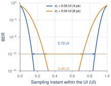
Jitter moves the crossings, so the BER also depends on when we sample. Sweeping the sampling instant across the UI gives a bathtub curve (Figure 2.12); its width at \(10^{-12}\) is the usable eye width. With 4 ps rms random jitter (0.02 UI), 0.72 UI remains; doubling the jitter leaves 0.45 UI. Chapter 11 covers this in full (Section 11.3).
Table 2.1. Q values for common BER targets. \(\mathrm{BER}= Q(x)\); \(2Q\) is the eye-to-noise ratio needed.
| BER | \(Q\) | \(2Q\) | SNR (dB) |
|---|---|---|---|
| \(10^{-3}\) | 3.09 | 6.18 | 9.8 |
| \(10^{-6}\) | 4.75 | 9.51 | 13.5 |
| \(10^{-9}\) | 6.00 | 12.00 | 15.6 |
| \(10^{-10}\) | 6.36 | 12.72 | 16.1 |
| \(10^{-12}\) | 7.03 | 14.07 | 16.9 |
| \(10^{-15}\) | 7.94 | 15.88 | 18.0 |
You cannot measure \(10^{-12}\) in a coffee break
Showing \(\mathrm{BER}< 10^{-12}\) at 95% confidence takes \(3/\mathrm{BER}= 3\times10^{12}\) error-free bits: ten minutes on the bench, far beyond any simulation. Design with statistical models; verify with PRBS checkers.
2.8Exercises
Rates. A 2.5GBASE-KX lane runs at 3.125 Gb/s with 8b/10b. Find \(T_\mathrm{b}\), \(f_\mathrm{N}\), the first PSD null and the payload rate.
PRBS9 (\(x^9 + x^5 + 1\)). Draw its LFSR; give its period, the counts of 1s and 0s, the longest runs and the line spacing at 5 Gb/s.
A CML stage as a pole. For \(R_\mathrm{L}= 200\,\Omega\), \(C_\mathrm{L}= 150\,\mathrm{fF}\), find \(f_\mathrm{3dB}\), \(t_r\) and \(1 - 2e^{-T_\mathrm{b}/\tau}\). What \(C_\mathrm{L}\) costs 10% of the eye?
Cursors by hand. With the cursors of Figure 2.6 (\(p_{-1}..p_{3}\) = 0.0205, 0.5561, 0.1605, 0.0629, 0.0340) and \(A = 0.5\,\mathrm{V}\), find the sample of the bracketed 1 in
1 1 1 [1] 0and in0 0 0 [1] 1. Compare the worst-case eye from these cursors with the 230 mV of the full tail.BER. A receiver sees \(\mathrm{EH} = 60\,\mathrm{mV}\) with \(\sigma_\mathrm{n}= 4\,\mathrm{mV}\). Find Q and the BER. What eye height or noise gives \(10^{-15}\), and how long must the link run error-free to show it?
Key takeaways
At 5 Gb/s, \(1\,\mathrm{UI}= 200\,\mathrm{ps}\) and \(f_\mathrm{N}= 2.5\,\mathrm{GHz}\); 77% of NRZ power lies below \(f_\mathrm{N}\).
PRBS-\(n\) (an \(n\)-stage LFSR) repeats every \(2^n - 1\) bits with runs up to \(n\); PRBS7 for bring-up, PRBS31 for compliance.
A one-pole block has \(t_r \approx 0.35/f_\mathrm{3dB}\) and a worst-case eye of \(2A(1 - 2e^{-T_\mathrm{b}/\tau})\); keeping ISI small needs \(f_\mathrm{3dB} \gtrsim f_\mathrm{N}\).
The received signal is \(y(t) = A\sum_n a_n\,p(t - nT_\mathrm{b})\): main cursor plus ISI from the cursors \(p_{k}\), with worst-case eye \(2A(p_{0} - \sum_{k\ne0}\lvert p_{k}\rvert)\).
With Gaussian noise, \(\mathrm{BER}= Q(\mathrm{EH}/2\sigma_\mathrm{n})\), so \(10^{-12}\) needs \(\mathrm{EH} \ge 14.07\,\sigma_\mathrm{n}\).
Generated from book/tutorial/chapters/02_signals.tex. Figure, table and equation numbers match the PDF edition.