Chapter 16Hands-on Labs with serdespy
Seven short Python scripts reproduce the key numbers of this tutorial, from the closed eye of the bare channel to a bang-bang CDR locking onto real data.
In this chapter you will learn
Set up serdespy on a current Python and run every lab from
tutorial/code/.Turn the REF channel into a pulse response, cursors and eye, and see why it must be equalized.
Design a TX FFE, a CTLE and a DFE in the model and measure what each buys.
Count bit errors with jitter and noise, and compare them with the semi-analytic BER and the bathtub.
Build a behavioral half-rate bang-bang PI-CDR and watch it track a frequency offset.
Every lab has the same shape: a goal, the few lines of code that matter, the figure and numbers you should get, and questions that push past the script. The figures here are drawn by figsrc/ch16_labN.py with exactly the computations of the labs, so your printed numbers must match to the last digit; each lab also writes its own PNGs.
16.1Lab 0: set-up
Goal
A working serdespy environment, and a map of the labs.
python3 -m venv ~/serdes-venv           # tested with Python 3.13
source ~/serdes-venv/bin/activate
pip install serdespy                     # pulls numpy, scipy, matplotlib, scikit-rf
cd tutorial/code
python lab1_channel.py                   # PNGs appear in this folder
serdespy 1.0 still uses np.complex_, which NumPy 2 removed; common.py, imported by every lab, restores it with np.complex_ = np.complex128 before serdespy is imported. It also defines the simulation grid (64 samples per UI, \(\Delta t=3.125\) ps, 0–160 GHz in 10 MHz steps) and the shared functions: channel() for REF, ctle(), impulse(), pulse(), tx_wave(), through(), the eye measurement eye_scan() (serdespy has none) and the Gaussian BER estimate ber_q(). Table 16.1 maps the labs to the chapters.
| Lab | Script | What it shows (key number) | Theory | Time |
|---|---|---|---|---|
| 1 | lab1_channel.py |
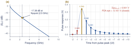
REF \(S_{21}\), \(h(t)\), \(p(t)\), cursors (\(-17.38\) dB; PDA \(-0.161\) V) | Sections 2.4 and 3.7 | 3 s |
| 2 | lab2_prbs_eye.py |
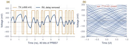
PRBS7 eye before and after REF (\(-77.8\) mV) | Section 2.6 | 2 s |
| 3 | lab3_tx_ffe.py |
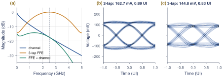
zero-forcing TX FFE (2-tap 162.7 mV, 3-tap 144.8 mV) | Chapter 6 | 3 s |
| 4 | lab4_ctle.py |
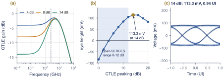
CTLE peaking sweep (113.3 mV at 14 dB) | Chapter 7 | 4 s |
| 5 | lab5_dfe.py |
DFE taps and BER (\(3.2\times10^{-14}\) at 10 mV) | Chapter 8 | 3 s |
| 6 | lab6_jitter_ber.py |
counted vs. estimated BER, bathtub (0.45 UI) | Chapter 11 | 21 s |
| 7 | lab7_bbcdr.py |
bang-bang PI-CDR (lock in 0.13 s, 0 errors) | Chapter 13 | 7 s |
serdespy quirks that cost an afternoon each
sdp.Transmitter(data, levels, f):fis the Nyquist frequency (pass 2.5e9 for 5 Gb/s), whatever the docstring says.Call
Transmitter.FIR()beforeoversample(), with taps[pre, main, post]or[main, post].sdp.channel_coefficients()always plots, at 1200 dpi by default: passres=150.sdp.forcing_ffe()sets the main tap to 1: rescale to \(\sum\lvert c_k\rvert=1\) yourself.Receiver.noise()discards any FFE or DFE already applied: add noise first, then equalize. UseReceiver.FFE(), notFFE_BR(), which misaligns the data.serdespy has no CDR and no MLSE, whatever the README lists; Lab 7 builds the CDR.
16.2Lab 1: the channel
Goal
Build REF from serdespy’s ABCD-matrix functions, plot \(\lvert S_{21}\rvert\), and turn it into the impulse response, the pulse response and its cursors (Sections 2.4 and 3.7).
from common import *

H = channel()                                  # complex S21 on the grid F
h, t = impulse(H)                              # h is per-sample: sum(h) = H(0)
p = pulse(h)
n_pre, n_post = 2, 10
cur = sdp.channel_coefficients(p, t, SPS, n_pre, n_post, res=150,
                               title="Pulse response and cursors")
isi = np.sum(np.abs(cur)) - cur[n_pre]
print(f"Peak-distortion eye (1 V swing, {n_pre}+{n_post} cursors) = "
      f"{cur[n_pre] - isi:+.4f} V  (negative = closed)")
What you should see
Figure 16.1. The loss is \(-0.59\) dB at DC, \(-10.40\) dB at 1.25 GHz, \(-17.38\) dB at 2.5 GHz and \(-30.07\) dB at 5 GHz. The cursors are \(p_{-1}=0.0486\), \(p_0=0.3396\), \(p_1=0.1817\), \(p_2=0.0909\), \(p_3=0.0537\) V, with \(p_1/p_0=0.535\). The ISI magnitudes add to 0.5008 V, more than the main cursor, so the peak-distortion eye is \(-0.161\) V: closed.
Questions and extensions
(1) Call channel(LOSS_FAMILY[10]) and channel(LOSS_FAMILY[25]) (0.572 and 1.441 m). How do \(p_1/p_0\) and the PDA eye change with loss? (2) Set c_pad=1e-12. Where in the tail do the pad reflections appear, and why can a short DFE not cancel them?
16.3Lab 2: a PRBS eye through the channel
Goal
Send PRBS7 NRZ through REF and measure the eye at both ends (Sections 2.2 and 2.6).
prbs = sdp.prbs7(1)                       # one period: 127 bits, seed = 1
bits = np.tile(prbs, 40)                  # 5080 bits = 1.016 us of data
tx = sdp.Transmitter(bits, LEVELS, F_NYQ)  # NB: 3rd argument = Nyquist frequency
tx.oversample(SPS)
x = tx.signal_ideal
H = channel()
h, t = impulse(H)
y = through(x, h)
hts_tx, ph_tx, _, _ = report_eye("TX output", x, bits)
hts_rx, ph_rx, S, A = report_eye("Channel output", y, bits)
save_eye(y, ph_rx, "Eye after 1 m channel (17.4 dB @ 2.5 GHz)", "lab2_eye_rx.png")
What you should see
Figure 16.2. The TX eye is 1000 mV and 1.00 UI. After REF the eye is \(-77.8\) mV and 0 UI wide: closed at every phase. The mean levels are \(+169.8\) and \(-165.3\) mV, at a best phase of 6/64 UI, and the channel delay is 6.722 ns.
Questions and extensions
(1) Repeat with sdp.prbs13(1) (tile it 2 times). Section 4.2 quotes \(-181\) mV: why is PRBS7 optimistic? (2) Count the longest run of identical bits in PRBS7 and in PRBS13. Which cursor sum does each run length expose?
16.4Lab 3: TX FFE
Goal
Compute zero-forcing 2-tap and 3-tap TX FFEs from the cursors, impose the peak-swing constraint, and measure the eyes (Chapter 6).
cur = sdp.channel_coefficients(p, t, SPS, 1, 1, res=150)
c3 = sdp.forcing_ffe(1, cur)              # [c-1, c0, c+1], c0 = 1
c3 = c3 / np.sum(np.abs(c3))              # peak-swing constraint sum|c| = 1
c2 = sdp.forcing_ffe(0, cur[1:])          # [c0, c+1]: classic de-emphasis
c2 = c2 / np.sum(np.abs(c2))
# ...
bits = np.tile(sdp.prbs7(1), 40)
for name, c, png in ((None, None, None), ("2-tap", c2, None),
                     ("3-tap", c3, "lab3_eye_ffe3.png")):
    y = through(tx_wave(bits, fir=c), h)
    hts, ph, S, A = report_eye(f"Channel + {name or 'no'} FFE", y, bits)
What you should see
Figure 16.3. The 3-tap taps are \([-0.0853, 0.5959, -0.3188]\) (DC gain 0.192, 14.34 dB of Nyquist boost), the 2-tap taps \([0.6515, -0.3485]\) (10.37 dB). The main cursor drops from 0.3396 to 0.1749 V, the price of equalizing at the TX. The eyes are 162.7 mV, 0.89 UI with 2 taps and 144.8 mV, 0.83 UI with 3 taps.
Questions and extensions
(1) Zero-forcing does not maximize the eye. Hold \(c_1\) and sweep \(c_{-1}\) from 0 to \(-0.1\), renormalizing each time: where is the best eye, and why does the pre-tap lose under \(\sum\lvert c_k\rvert=1\)? (2) Quantize the taps to multiples of 1/32 (the 5-bit driver of Section 9.5). How much eye is lost?
16.5Lab 4: CTLE
Goal
Sweep the peaking of a one-zero, two-pole CTLE, find the best eye, and translate it into a degenerated differential pair (Section 7.2).
FP1, FP2 = 2.5e9, 10e9                    # pole 1 at Nyquist, output pole 10 GHz
H = channel()
bits = np.tile(sdp.prbs7(1), 40)
x = tx_wave(bits)
peaks, eh, ew = np.arange(0, 21, 2), [], []
for pk in peaks:
    h_link, t = impulse(H * ctle(pk, FP1, FP2))   # channel x CTLE
    hts, ph, S, A = eye_scan(through(x, h_link), bits)
    eh.append(hts[ph]); ew.append(np.sum(hts > 0) / SPS)
best = peaks[int(np.argmax(eh))]
# ...
gm, a = 20e-3, 10**(best / 20)            # example: gm = 20 mS per side
RS = 2 * (a - 1) / gm                     # A = 1 + gm*RS/2
CS = 1 / (RS * 2 * np.pi * FP1 / a)       # wz = 1/(RS*CS)
RD, CL = 1 / gm, 1 / (2 * np.pi * FP2 / gm)   # gm*RD = 1, wp2 = 1/(RD*CL)
What you should see
Figure 16.4. The eye opens at 6 dB (31.6 mV), reaches 104.0 mV at 12 dB, peaks at 113.3 mV, 0.94 UI at 14 dB and falls again beyond. With 14 dB nominal, the real peak-to-DC gain is only 12.11 dB because the second pole eats some of it; the CTLE is \(-14.00\) dB at DC and \(-3.10\) dB at Nyquist. The circuit values are \(R_S=401\,\Omega\), \(C_S=0.795\) pF, \(R_D=50\,\Omega\) and \(C_\mathrm{L}=318\) fF.
Questions and extensions
(1) The optimum lies outside the Open-SERDES range. What does the DFE of Lab 5 do with the 8 dB eye that the CTLE alone cannot? (2) Move FP2 to 6 GHz and re-sweep; compare with Worked Example 15.1.
16.6Lab 5: DFE
Goal
Take the post-cursors left by a moderate 8 dB CTLE as DFE taps, measure the eye against the number of taps, and estimate the BER (Chapter 8).
PEAK = 8                                   # CTLE peaking [dB] (lab 4 model)
h_link, t = impulse(H * ctle(PEAK))        # channel x CTLE
y = through(tx_wave(bits), h_link)         # CTLE output waveform
cur = sdp.channel_coefficients(pulse(h_link), t, SPS, 1, 8, res=150)
h_pre, h0, post = cur[0], cur[1], cur[2:]
for n in (0, 1, 2, 3, 4, 5, 8):
    rx = sdp.Receiver(y, SPS, F_NYQ, LEVELS, shift=True)  # centre eye at 0
    if n:
        rx.nrz_DFE(post[:n])
    report_eye(f"CTLE {PEAK} dB + {n}-tap DFE", rx.signal, bits)
# ... final design: 3 taps, then ber_q(S[ph], A[ph], sigma) for 5..20 mV
What you should see
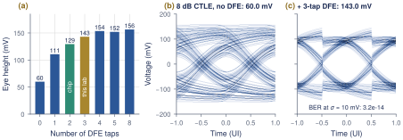
Figure 16.5. With the 8 dB CTLE, \(p_{-1}=0.0138\), \(p_0=0.1832\) and \(p_1\)–\(p_3\) = 0.0552, 0.0235, 0.0160 V. The eye grows from 60.0 mV with no DFE to 110.7, 129.5 and 143.0 mV with 1, 2 and 3 taps, then saturates near 155 mV. With 3 taps the feedback is \(\pm27.6\), \(\pm11.8\) and \(\pm8.0\) mV, and the estimated BER is \(5.9\times10^{-46}\), \(3.2\times10^{-14}\), \(6.0\times10^{-8}\) and \(1.8\times10^{-5}\) at \(\sigma\) = 5, 10, 15 and 20 mV. A noise-free run through sdp.prbs_checker gives 0 errors in 5024 bits. The lab uses 3 taps; the chip has 2, which gives 129.5 mV here.
Questions and extensions
(1) Reproduce the Open-SERDES operating point of Section 8.5: TX taps \([0.75, -0.25]\) (\(-6\) dB), a 0 dB CTLE and 2 DFE taps. You should get 171.8 mV. (2) The worst-case \(Q\) at 10 mV is \(143.0/2/10=7.15\), yet the BER is \(3.2\times10^{-14}\), not \(Q(7.15)\). Why is ber_q more optimistic than the worst case?
16.7Lab 6: jitter, noise and BER
Goal
Add 5 ps rms TX random jitter and RX noise to the Lab 5 link, count real bit errors, and compare them with the estimate and the bathtub (Section 11.3).
np.random.seed(2026)                       # repeatable jitter and noise
PEAK, N_TAPS, RJ_UI = 8, 3, 0.025          # RJ = 2.5 % UI = 5 ps rms
bits = np.tile(sdp.prbs7(1), 800)          # 101 600 bits
y = through(tx_wave(bits, jitter_ui=RJ_UI), h_link)   # TX RJ -> channel -> CTLE
rx = sdp.Receiver(y, SPS, F_NYQ, LEVELS, shift=True)  # sampling phase -> index 0
rx.nrz_DFE(taps)
hts, ph, S, A = report_eye("With 5 ps TX RJ, no noise", rx.signal, bits)
for sigma in (10e-3, 15e-3, 20e-3, 25e-3):
    rx.noise(sigma)                        # resets to pre-DFE signal + AWGN
    rx.nrz_DFE(taps)                       # real decisions: error propagation
    d = sdp.nrz_a2d(rx.signal, SPS, 0.0)[skip:-5]
    n_err = sdp.prbs_checker(7, sdp.prbs7(1), d)[0]
    est = ber_q(S[0], A[0], sigma)
# ... bathtub: ber_q(S[o % SPS], A[o % SPS], sigma) at every phase offset o
What you should see
Figure 16.6. With jitter but no noise the eye is 115.6 mV and 0.73 UI. Counting over 101 544 bits:
| \(\sigma\) (mV) | 10 | 15 | 20 | 25 |
|---|---|---|---|---|
| errors counted | 0 | 1 | 6 | 43 |
| counted BER | \(<3\times10^{-5}\) | \(9.9\times10^{-6}\) | \(5.9\times10^{-5}\) | \(4.2\times10^{-4}\) |
| estimated BER | \(1.4\times10^{-12}\) | \(1.4\times10^{-7}\) | \(2.4\times10^{-5}\) | \(3.9\times10^{-4}\) |
At 25 mV count and estimate agree within 10 %; the single 15 mV error is a true rare event (a 63.6 mV margin hit by \(4.25\sigma\) of noise). With \(\sigma=5\) mV the bathtub is open 0.45 UI at \(10^{-12}\) (0.66 UI at \(10^{-5}\)); at 20 mV it never reaches \(10^{-5}\), and the counted points fall on the estimate.
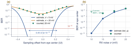
ber_q for 5 and 20 mV of noise, with error counts at 20 mV (dots) at offsets up to \(\pm0.375\) UI. (b) BER at the eye center against noise. The open triangle at 10 mV is the 95 % bound \(3/N\) of Equation (15.4) for zero errors in \(N\) bits.Questions and extensions
(1) How many bits would you have to simulate to see one error at \(\sigma=10\) mV? How long would that take? (2) Raise the RJ to 6 ps rms (RJ_UI = 0.03). How much does the \(10^{-12}\) opening at 5 mV shrink? Compare with the 14\(\sigma\) rule of Equation (11.3).
16.8Lab 7: a bang-bang PI-CDR
Goal
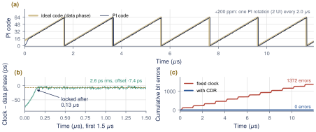
serdespy has no CDR, so lab7_bbcdr.py builds one on the Lab 4 link (REF + 14 dB CTLE, 5 ps RJ, 5 mV noise): a half-rate Alexander detector, a P+I loop filter at 625 MHz and a 64-step PI, with the RX clock 200 ppm fast and starting 74 ps off the eye center, as in Figure 13.9. It samples the real waveform where the PI says: per UI one data sample D and one edge sample E half a UI earlier, as the four half-rate samplers deliver. A transition with \(E\) equal to the previous \(D\) means the clock is early (the loop body below is excerpted; the script also counts errors and has a fixed-clock mode).
for k in range(n_upd):
    n = k * UPD + np.arange(UPD)                      # RX bit indices of this update
    # ... phi_d = data phase: phi0 + ppm offset + optional sinusoidal jitter
    phi_c = np.round(acc) * LSB                       # PI phase (UI)
    t_d = t0 + SPS * (n - phi_d + phi_c)              # data-sampler instants
    d = sample(y, t_d) + sigma * rng.standard_normal(UPD) > 0
    e = sample(y, t_d - SPS / 2) + sigma * rng.standard_normal(UPD) > 0
    prev = np.concatenate(([d[0] if d_prev is None else d_prev], d[:-1]))
    trans = prev != d                                 # a transition before each bit
    votes = np.where(e == prev, 1, -1) * trans        # +1: clock early -> later
    pipe.append(np.sign(votes.sum()))                 # majority vote of the block
    v = pipe.pop(0)                                   # ... seen d_lat updates later
    if cdr:
        freg += ki * v                                # integral path (frequency)
        acc += kp * v + freg                          # proportional path + phase
What you should see
Figure 16.7, with the baseline of Section 13.6 (\(K_P\) = 1/8 LSB, \(K_P/K_I\) = 128, one update of extra latency). The loop locks in 0.13 s (the phase-only model of Figure 13.9, with a stricter lock test, reports 0.19 s); the integral register settles at 199 ppm against the true 200; the tracking error is 2.57 ps rms and 17.3 ps peak-to-peak, around a static offset of \(-7.4\) ps from the maximum-height eye center. There are 0 bit errors in 59 680 bits with the CDR, against 1372 (BER \(2.3\times10^{-2}\)) with a fixed clock, which slides across an eye edge once per microsecond. Raising \(K_P\) to 1/2 and 1 LSB raises the wander to 5.13 and 9.90 ps rms (31.1 and 57.5 ps pp): the trade-off of Worked Example 13.2.
Questions and extensions
(1) Sweep \(K_P\) from 1/16 to 1 LSB and the latency d_lat from 0 to 4. Plot the rms and peak-to-peak wander and compare with dither \(\approx2S\,T_\mathrm{lat}\) (Section 13.4). (2) Set ki=0 and raise ppm to 300, 450 and 550. Where does the proportional-only loop lose lock, and does it match the 488 ppm of Section 13.6? Watch the static phase offset grow with the frequency offset before it fails. (3) Add sinusoidal jitter with sj_pp and sj_f. Find the largest amplitude at 1 and 4.9 MHz with zero errors, and plot your JTOL points on Figure 13.6. Why does the loop lock 7 ps before the eye center?
16.9Where to go next
Build the GUI demo
The proposal lists a GUI front-end for the link model among its deliverables, in the spirit of the Julia SerDes framework (JLSD) [64] it cites. The labs are the engine: put sliders for loss, taps, peaking and noise in front of channel(), the FFE, ctle(), the DFE and lab7_bbcdr.simulate(), and redraw the eye and bathtub on every change. Cross-check the eyes against PyBERT [44], a mature open link simulator with IBIS-AMI support.
Use a measured channel
Load the test board’s 4-port Touchstone file. sdp.four_port_to_diff assumes ports 1\(\to\)2 and 3\(\to\)4 and returns \(V_\mathrm{out}/V_s\), half of \(S_{21}\) for a matched link; the data must start near DC (scikit-rf can extrapolate).
import skrf as rf
ntw = rf.Network("board.s4p")               # measured channel, ports 1->2, 3->4
Hd, fd, hd, td = sdp.four_port_to_diff(ntw, None, 50, 50, t_d=DT)
h = 2 * hd                                  # S21-like: same scale as impulse(channel())
On a synthetic 4-port built from REF this returns exactly \(-17.38\) dB and \(p_0=0.3396\) V; Labs 2–7 then run unchanged. Next: crosstalk, adaptation with sdp.lms_equalizer, and the statistical eye of Section 4.3.
Key takeaways
serdespy 1.0 runs on NumPy 2 with one shim; remember its quirks: Nyquist frequency in
Transmitter, FIR before oversampling,res=150, renormalized taps, noise before equalization.REF loses 17.38 dB at Nyquist; its PDA eye is \(-0.161\) V and its PRBS7 eye \(-77.8\) mV.
Under the peak-swing constraint the 2-tap FFE (162.7 mV) beats the zero-forcing 3-tap (144.8 mV); a CTLE alone peaks at 113.3 mV at 14 dB; 8 dB plus a 2- or 3-tap DFE gives 129.5 or 143.0 mV.
Counted errors confirm
ber_qwhere counting is possible; below \(10^{-5}\) only the estimate speaks.A bang-bang PI-CDR locks to 200 ppm in 0.13 s with 2.6 ps rms wander and no errors (a fixed clock: 1372).
Generated from book/tutorial/chapters/16_labs.tex. Figure, table and equation numbers match the PDF edition.