Chapter 11Jitter
A 200 ps bit leaves no room for sloppy clock edges: this chapter turns “the clock wobbles” into numbers you can budget, measure and design against.
In this chapter you will learn
Define time-interval error, period jitter and cycle-to-cycle jitter, and say which one a serial link cares about.
Convert voltage noise into timing jitter through the slew rate.
Separate random from deterministic jitter and combine them with the dual-Dirac model, \(\mathrm{TJ} = \mathrm{DJ}_{\delta\delta} + 2Q\,\sigma_\mathrm{RJ}\).
Integrate a phase-noise spectrum \(\mathcal{L}(f)\) into rms jitter with the right limits.
Build the Open-SERDES jitter budget and check it against 0.3 UI at \(10^{-12}\).
11.1What jitter is
An ideal clock has edges at exactly \(t = nT\); a real clock has edges at \(t_n\), each a little early or late. Jitter is that deviation. Three measures are in common use (Figure 11.1a): \[\mathrm{TIE}_n = t_n - nT, \qquad J_{\mathrm{per},n} = T_n - T = \mathrm{TIE}_{n+1} - \mathrm{TIE}_n, \qquad J_{\mathrm{cc},n} = T_{n+1} - T_n , \tag{11.1}\] where \(T_n = t_{n+1} - t_n\) is the \(n\)-th period. The time-interval error (TIE, also called absolute jitter) is the one a link cares about, because the sampler compares a clock edge with a data edge, not one clock period with the next. Period jitter and cycle-to-cycle jitter matter for digital setup and hold, but they can be tiny while the TIE is large, because small period errors add up.
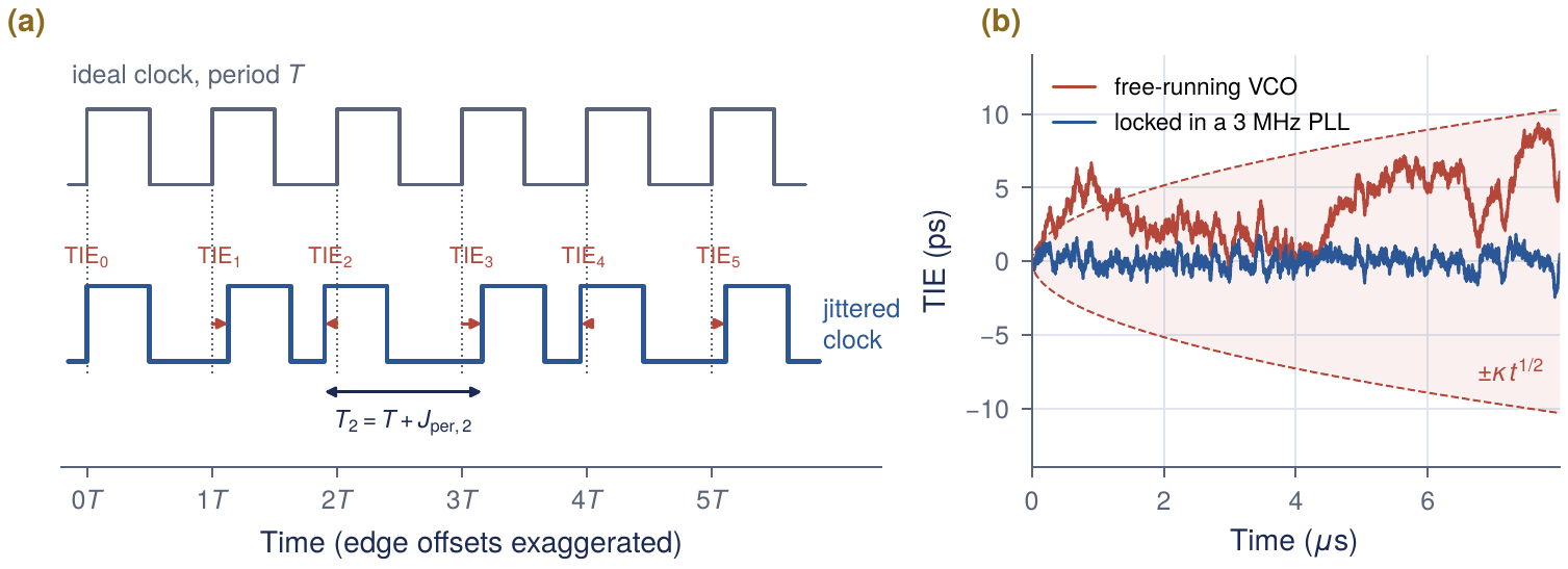
Figure 11.1(b) shows the difference. A free-running oscillator has no memory of where its edges should be, so its TIE random-walks. A phase-locked loop (Chapter 12) compares its edges with a clean reference and keeps the TIE bounded. The CDR (Chapter 13) does the same for the data: it tracks slow jitter and leaves only the fast part to close the eye.
Worked Example 11.1 · Three jitter numbers from six edges
Given: \(T = 400\) ps and edges at 0, 401.0, 799.5, 1201.5, 1600.0 and 2000.8 ps. TIE: 0, 1.0, \(-0.5\), 1.5, 0, 0.8 ps: 2.0 ps peak-to-peak, 0.69 ps rms about the mean. Period jitter: 1.0, \(-1.5\), 2.0, \(-1.5\), 0.8 ps: 1.42 ps rms. Cycle-to-cycle: \(-2.5\), 3.5, \(-3.5\), 2.3 ps: 3.0 ps rms.
Lesson: \(J_\mathrm{cc} > J_\mathrm{per} > \mathrm{TIE}\) is typical of a locked clock: a bounded TIE means a long period is usually followed by a short one. Always say which measure a number is.
Voltage noise becomes timing noise
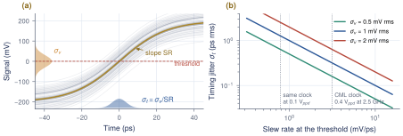
Near a threshold crossing, a noise voltage moves the crossing by the noise divided by the slope of the edge (Figure 11.2a):
Key equation · Noise-to-jitter conversion
\[\sigma_t = \frac{\sigma_v}{\mathrm{SR}}, \qquad \mathrm{SR} = \left.\frac{dv}{dt}\right|_\text{crossing} = 2\pi f_0 A_c \ \text{for a sine of amplitude } A_c . \tag{11.2}\]
A 2.5 GHz CML clock of 0.4 V\(_\mathrm{ppd}\) (\(A_c = 0.2\) V) slews at 3.14 mV/ps, so 1 mV rms of noise costs 0.32 ps rms. Attenuated to 0.1 V\(_\mathrm{ppd}\) by a lossy route, the same clock turns the same noise into 1.27 ps (Figure 11.2b). The relation also works in reverse: Section 2.6 showed that sampling a few picoseconds off the eye centre costs millivolts.
Design rule of thumb
Keep clock swings large and edges fast wherever a clock is buffered or sampled: halving the slew rate doubles the jitter from the same noise. This is why Open-SERDES restores its 2.5 GHz clocks with CML limiting buffers (Section 12.5) instead of letting them decay along long wires.
11.2Random and deterministic jitter
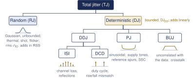
Jitter sources fall into two families with different statistics (Figure 11.3). Random jitter (RJ) comes from thermal, shot and flicker noise. It is Gaussian and unbounded, and is described by its rms \(\sigma_\mathrm{RJ}\); a peak-to-peak RJ is meaningless without a BER. Deterministic jitter (DJ) is bounded. Its parts are data-dependent jitter (DDJ), mainly ISI from the channel plus duty-cycle distortion (DCD); periodic jitter (PJ) from supply tones, reference spurs or spread-spectrum clocking, whose arcsine PDF piles up at its peaks; and bounded uncorrelated jitter (BUJ), mostly crosstalk.
After Palermo [34].
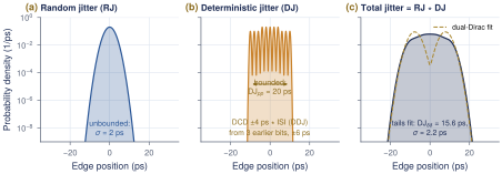
When independent sources act on the same edge, the PDF of the total is the convolution of their PDFs, the rule Section 4.3 used for ISI. In Figure 11.4 a 2 ps RJ convolved with 20 ps\(_\mathrm{pp}\) of DJ gives a total whose centre looks like the DJ and whose tails are Gaussian.
11.3The dual-Dirac model and total jitter
At \(10^{-12}\) only the far tails of the jitter PDF matter. The dual-Dirac model [21] keeps the tails and simplifies the rest: all DJ becomes two impulses at \(\pm\mathrm{DJ}_{\delta\delta}/2\), each carrying a Gaussian of rms \(\sigma_\mathrm{RJ}\) (Figure 11.5a).
From two Gaussians to total jitter
Measure the sampling instant \(x\) from the left crossing of the eye. Far out, only the Gaussian centred at \(+\mathrm{DJ}_{\delta\delta}/2\) can put an edge later than \(x\), with probability \(Q\big((x - \mathrm{DJ}_{\delta\delta}/2)/\sigma_\mathrm{RJ}\big)\). Adding the mirror image from the right crossing gives the bathtub curve \[\mathrm{BER}(x) \approx Q\!\left(\frac{x - \mathrm{DJ}_{\delta\delta}/2}{\sigma_\mathrm{RJ}}\right) + Q\!\left(\frac{\mathrm{UI}- x - \mathrm{DJ}_{\delta\delta}/2}{\sigma_\mathrm{RJ}}\right).\] The target BER is reached where \(x - \mathrm{DJ}_{\delta\delta}/2 = Q_\mathrm{BER}\,\sigma_\mathrm{RJ}\) on each side, with \(Q(Q_\mathrm{BER}) = \mathrm{BER}\). The eye that remains is \(\mathrm{UI}- \mathrm{DJ}_{\delta\delta} - 2Q_\mathrm{BER}\,\sigma_\mathrm{RJ}\); the rest is total jitter.
Key equation · Total jitter at a BER (dual-Dirac)
\[\mathrm{TJ}(\mathrm{BER}) = \mathrm{DJ}_{\delta\delta} + 2\,Q_\mathrm{BER}\,\sigma_\mathrm{RJ}, \qquad \text{eye width} = 1\,\mathrm{UI}- \mathrm{TJ}, \qquad 2Q_{10^{-12}} = 14.07 . \tag{11.3}\]
\(Q_\mathrm{BER}\) is the Gaussian quantile of Equation (2.9): 6.00 at \(10^{-9}\), 7.03 at \(10^{-12}\), 7.94 at \(10^{-15}\). The derivation drops two factors of \(\tfrac12\) (each impulse carries half the edges, and about half the bits have no transition); keeping them gives \(Q = 6.84\). The industry keeps 7.03, which is 3% conservative, and so do we.
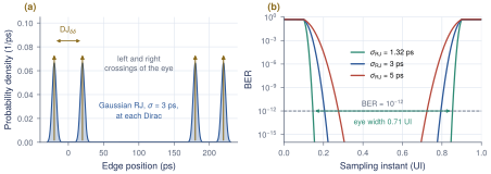
Figure 11.5(b) completes the teaser of Section 2.7. Note the factor 14.07 in Equation (11.3): a picosecond of RJ costs 14 ps of eye at \(10^{-12}\), while a picosecond of DJ costs one.
DJ\(_{\delta\delta}\) is not DJ\(_\mathrm{pp}\)
DJ\(_{\delta\delta}\) is a model parameter fitted to the tails. It is smaller than the true peak-to-peak DJ unless the DJ is two-valued, such as pure DCD (15.6 versus 20 ps in Figure 11.4). Use DJ\(_{\delta\delta}\) in Equation (11.3), and fit the tails at deep BER (Q of 4 or more): a fit at \(10^{-3}\) overestimates \(\sigma_\mathrm{RJ}\). A direct TJ(\(10^{-12}\)) measurement needs about \(10^{13}\) bits, half an hour per point at 5 Gb/s.
11.4From phase noise to jitter
Oscillators are specified in the frequency domain. The single-sideband phase noise \(\mathcal{L}(f)\) is the noise power in 1 Hz at offset \(f\) from the carrier, relative to the carrier, in dBc/Hz. For small noise it is half the one-sided phase spectrum \(S_\phi(f)\), so integrating it gives the phase variance, and dividing by \(2\pi f_0\) turns phase into time:
Key equation · Phase noise to rms jitter
\[\sigma_t = \frac{\sigma_\phi}{2\pi f_0} = \frac{1}{2\pi f_0}\sqrt{2\!\int_{f_1}^{f_2}\!\mathcal{L}(f)\,df}, \qquad \mathcal{L} \text{ in linear units } \big(10^{\mathcal{L}_\mathrm{dB}/10}\big). \tag{11.4}\]
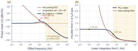
The limits matter. The upper limit \(f_2\) is about \(f_0/2\). The lower limit \(f_1\) is set by what the receiver tracks: jitter far below the CDR bandwidth moves the clock and the data together and does not close the eye. Integrating from 10 kHz gives the clock’s absolute jitter; integrating from the CDR bandwidth gives the jitter that reaches the sampler (Figure 11.6).
A useful shortcut
In the \(1/f^2\) region of an LC oscillator, \(\mathcal{L}(f) = \mathcal{L}(\Delta f)(\Delta f/f)^2\), and the free-running TIE grows as \(\kappa\sqrt{t}\) with \(\kappa = (\Delta f/f_0)\sqrt{\mathcal{L}(\Delta f)}\). If a loop tracks this noise below a corner \(f_c\) (a first-order high-pass), Equation (11.4) integrates in closed form to \[\sigma_t \approx \kappa/\sqrt{4\pi f_c} , \tag{11.5}\] so jitter falls only as \(1/\sqrt{f_c}\): quadrupling the bandwidth halves the VCO’s share.
Worked Example 11.2 · Phase noise of the team PLL as jitter
Given: \(\mathcal{L} = -100.8\) dBc/Hz at 1 MHz [9], applied at \(f_0 = 2.5\) GHz. Assumptions (they change the answer): the value describes the free-running VCO with a \(1/f^2\) slope and a 100 kHz \(1/f^3\) corner; the in-band floor from reference and charge pump is \(-110\) dBc/Hz; the PLL is the 3 MHz design of Section 12.2.
Free-running: \(\mathcal{L} = 8.3\times10^{-11}\), so \(\kappa = 4\times10^{-4}\sqrt{8.3\times10^{-11}} = 3.65\times10^{-9}\,\sqrt{\mathrm{s}}\). Period jitter \(\kappa\sqrt{400\,\mathrm{ps}} = 73\) fs; TIE after 1 s \(= 3.65\) ps. Locked, shortcut: \(3.65\times10^{-9}/\sqrt{4\pi\times3\,\mathrm{MHz}} = 0.59\) ps from the VCO. Locked, full model (Figure 11.6): 1.01 ps rms from 10 kHz, 0.61 ps above 4 MHz.
Check the assumption: Section 12.4 shows that a \(Q = 16.8\) tank should be about 20 dB quieter than \(-100.8\) dBc/Hz, so the number may be a closed-loop value. If so, every VCO term here is pessimistic. Confirm with the team before freezing the PLL bandwidth.
11.5The Open-SERDES jitter budget
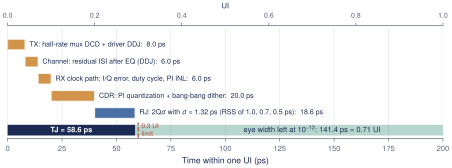
A jitter budget divides the UI among the blocks that move edges, so each designer gets a number to meet. Add DJ\(_{\delta\delta}\) linearly, add RJ in RSS, and combine with Equation (11.3). The Open-SERDES target is TJ \(\le\) 0.3 UI = 60 ps at \(10^{-12}\), measured at the sampler; the remaining 0.7 UI covers the sampler aperture and setup time (Section 10.2), static phase offsets and margin. Only jitter the CDR does not track is counted: the clock RJ rows use the phase noise above the CDR bandwidth (0.61 ps from Worked Example 11.2, rounded up to cover the buffers), and the CDR row is the CDR’s own tracking error (Table 11.1, Figure 11.7).
| Contributor | DJ\(_{\delta\delta}\) (ps) | RJ (ps rms) | Owner |
|---|---|---|---|
| TX: half-rate mux DCD, driver data-dependent jitter | 8 | – | Chapter 9 |
| Channel: residual ISI after equalization (DDJ) | 6 | – | Chapter 8 |
| RX clock path: I/Q error, duty cycle, PI nonlinearity | 6 | – | Section 12.5 |
| CDR: PI quantization and bang-bang dither | 20 | – | Section 13.6 |
| TX clock: PLL plus buffers, not tracked by the CDR | – | 1.0 | Chapter 12 |
| RX clock: PLL, PI and buffers, not tracked | – | 0.7 | Chapter 12 |
| Samplers: aperture and noise | – | 0.5 | Section 10.2 |
| Total | 40 | 1.32 (RSS) |
Worked Example 11.3 · Does the budget close?
DJ: \(8 + 6 + 6 + 20 = 40\) ps. RJ: \(\sigma = \sqrt{1.0^2 + 0.7^2 + 0.5^2} = 1.32\) ps, so \(2Q\sigma = 14.07\times1.32 = 18.6\) ps. TJ: \(40 + 18.6 = \mathbf{58.6}\) ps \(=\) 0.293 UI, inside 0.3 UI with 1.4 ps to spare; the eye at \(10^{-12}\) is 141 ps wide.
Turn it around: with DJ at 40 ps, RJ may be at most \((60-40)/14.07 = 1.42\) ps rms; with RJ fixed, DJ may grow by only 1.4 ps. Tight budgets are normal. Consistency: Section 4.3 used 2 ps RJ and 20 ps DJ for the sampling clock; the CDR row here is that 20 ps, and 2 ps conservatively covers the RX share of the RJ.
What this means for your design
The largest line is the CDR’s own dither, and the most expensive per picosecond is RJ, because of the factor 14. So: design the CDR loop for low dither (Section 13.6); keep the PLL’s untracked jitter below 1 ps rms (Chapter 12); and keep duty-cycle and quadrature errors small, because they become DJ at the half-rate samplers (Section 12.5).
11.6Jitter transfer, generation and tolerance
Three more terms describe how a block treats jitter versus jitter frequency. Jitter transfer is the ratio of output to input jitter: a PLL is low-pass to its reference, a CDR low-pass to the data. Jitter generation is the jitter a block adds with a clean input. Jitter tolerance (JTOL) is the largest sinusoidal jitter a receiver can take at a given frequency and still meet the BER. Because the CDR tracks slow jitter, a receiver tolerates many UI at low frequency but only its eye margin at high frequency; Section 13.5 checks the Open-SERDES CDR against a mask.
Lab 6: jitter and the bathtub
Section 16.7 adds RJ and DJ to the REF link and plots the bathtub. Reproduce Figure 11.5(b), then change \(\sigma_\mathrm{RJ}\) by 0.5 ps and watch the eye width move by 7 ps.
Key takeaways
A link cares about time-interval error, and only the part the CDR does not track.
Voltage noise becomes jitter through the slope, \(\sigma_t = \sigma_v/\mathrm{SR}\): keep clock swings large and edges fast.
RJ is Gaussian and unbounded (rms, adds in RSS); DJ is bounded (DDJ, DCD, PJ, BUJ; adds linearly). Their PDFs convolve.
Dual-Dirac: \(\mathrm{TJ} = \mathrm{DJ}_{\delta\delta} + 2Q\sigma_\mathrm{RJ}\) with \(2Q = 14.07\) at \(10^{-12}\); one picosecond of RJ costs 14 ps of eye.
\(\sigma_t = \sqrt{2\int\mathcal{L}\,df}/(2\pi f_0)\), integrated from the CDR bandwidth. The team PLL model gives 1.01 ps from 10 kHz and 0.61 ps above 4 MHz.
The Open-SERDES budget (40 ps DJ, 1.32 ps RJ) gives TJ = 58.6 ps = 0.293 UI against 0.3 UI; the CDR’s 20 ps is the largest line.
Generated from book/tutorial/chapters/11_jitter.tex. Figure, table and equation numbers match the PDF edition.