Chapter 9The Transmitter
Sixteen slow bits go in, one fast differential wave comes out: the serializer, the termination, the CML driver with its FFE, and the pad that connects them to the channel.
In this chapter you will learn
Explain with the FO4 rule why the last serializer stages and their clocks must be half-rate CML in 130 nm.
Design an HBT CML 2:1 multiplexer and read its timing, including duty-cycle errors.
Compare series, parallel and double termination, and compute what double termination costs.
Size the Open-SERDES CML driver (current, swing, power, headroom, \(\mathrm{BV}_\mathrm{CEO}\)) and compare it with a voltage-mode driver.
Build the 3-tap FFE as a current-summing driver and choose its tap resolution.
Budget the pad, ESD and driver capacitance, and decide when a T-coil is worth its area.
9.1The transmitter at a glance
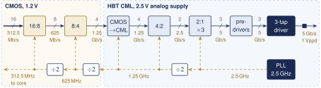
The transmitter takes a 16-bit word from the digital core every 3.2 ns (312.5 MHz) and launches it as a 5 Gb/s NRZ wave into the 50 Ω-per-side channel (Figure 9.1). Each 2:1 stage doubles the lane rate and is clocked at half its output bit rate. The clocks come from the 2.5 GHz PLL (Chapter 12) through a chain of \(\div2\) dividers. Static CMOS on 1.2 V handles the slow, wide part. HBT current-mode logic (CML) on the 2.5 V analog supply handles everything at 1.25 GHz and above. The final 2:1 multiplexer is built three times, so that the driver receives \(D_{n+1}\), \(D_n\) and \(D_{n-1}\) for its three FFE taps.
9.2The serializer
9.2.1Clocks, not gates, set the speed
A 130 nm CMOS gate switches in tens of picoseconds, yet a 5 GHz CMOS serializer does not work, because the clock has to be distributed. A clock passing through a chain of inverters keeps its shape only if each half-period lets every inverter swing fully. Below about 8 fan-out-of-4 delays per period, the pulses shrink at each stage and vanish [24]. The FO4 delay \(t_\mathrm{FO4}\), the delay of an inverter driving four copies of itself, is the natural unit of CMOS speed.
Key equation · The clock-distribution limit
\[T_\mathrm{clk}\ \ge\ 8\,t_\mathrm{FO4}\qquad\Longrightarrow\qquad f_\mathrm{b}\le \frac{n}{8\,t_\mathrm{FO4}}, \tag{9.1}\] where \(n\) is the number of bits per clock period: 1 at full rate, 2 at half rate, 4 at quarter rate.
Worked Example 9.1 · Can CMOS clock the last stage?
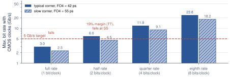
Given: \(t_\mathrm{FO4}\approx42\,\mathrm{ps}\) for 1.2 V SG13G2 CMOS at the typical corner and about 55 ps at the slow corner. These are 130 nm estimates: measure yours in ngspice with a chain of inverters, each loaded by four copies of itself.
Full rate needs \(T_\mathrm{clk}=200\,\mathrm{ps}=4.8\,t_\mathrm{FO4}\), and Equation (9.1) allows only 3.0 Gb/s. Half rate needs \(T_\mathrm{clk}=400\,\mathrm{ps}\): \(9.5\,t_\mathrm{FO4}\) typical but \(7.3\,t_\mathrm{FO4}\) slow, a limit of 5.95 and 4.55 Gb/s. CMOS fails at the slow corner (Figure 9.2).
Conclusion: the final 2:1 stage and its clock must be CML, whose speed is set by \(R_\mathrm{L}C_\mathrm{L}\) rather than FO4. Stages at 625 MHz and below (\(T_\mathrm{clk}\ge29\,t_\mathrm{FO4}\)) stay in CMOS.
9.2.2The half-rate CML 2:1 multiplexer
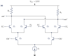
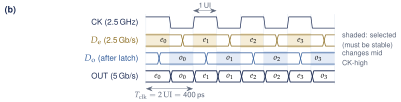
A half-rate multiplexer has no full-rate flip-flop at its output. The clock itself is the select: the even bit goes out while CK is high and the odd bit while CK is low [24]. Figure 9.3(a) shows the HBT version, a stacked (series-gated) CML gate. The clock pair \(Q_5/Q_6\) steers the tail current \(I_T\) into one of the two data pairs, and the selected pair steers it into one of the shared loads \(R_\mathrm{L}\). The deselected pair carries no current. The data bases sit at CML levels and the clock bases one \(V_\mathrm{BE}\) lower, through emitter followers, so every device keeps its \(V_\mathrm{CE}\) near 0.8 V on the 2.5 V supply.
Key equation · CML gate design
\[\Delta V = I_TR_\mathrm{L},\qquad \tau=R_\mathrm{L}C_\mathrm{L},\qquad P = V_\mathrm{CC}I_T=\frac{V_\mathrm{CC}\,\Delta V\,C_\mathrm{L}}{\tau}. \tag{9.2}\] Choose the swing \(\Delta V\) first, then \(R_\mathrm{L}\) from the speed target \(\tau\), then \(I_T\).
Glitch-free timing and retiming
The select must never switch while a selected input changes. In Figure 9.3(b) each input changes in the middle of the half where it is deselected: the even data directly, the odd data after one extra latch. Data from the 4:2 stage, which runs on the divided 1.25 GHz clock, is retimed by latches on the 2.5 GHz clock, and transitions placed mid-way through the deselected half leave \(\pm100\,\mathrm{ps}\) for divider delay, wiring, setup and hold (800 ps at the CMOS-to-CML boundary). A skew beyond the window does not degrade the eye gracefully: it shifts the bits by one position.
Duty cycle becomes UI width
A clock with duty cycle \(D\) produces even UIs of \(2DT_\mathrm{b}\) and odd UIs of \(2(1-D)T_\mathrm{b}\). A 45 % duty cycle gives alternating 180 and 220 ps bits, 20 ps of deterministic jitter before the channel acts (Chapter 11). Restore the clock to 50 % with a CML buffer chain or a duty-cycle corrector right before the mux.
What this means for your design
Build the last two serializer stages and the 2.5 GHz clock buffers in HBT CML, and everything from 625 MHz down in 1.2 V CMOS. Half rate removes the 5 GHz clock but turns duty cycle into UI width: budget for a duty-cycle corrector, and simulate every clock-domain boundary at all corners.
9.3Termination
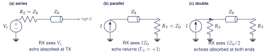
A wave that meets an impedance step reflects (Section 3.4). A link can absorb it at the source, at the load or at both ends (Figure 9.4).
Why double termination wins
Nothing is perfectly matched: pad capacitance, resistor tolerance and the package always reflect a few percent of the wave at the RX. With \(R_S=Z_0\) that echo dies at the TX (\(\Gamma_S=0\)) instead of returning as a delayed copy of the bit, which would be ISI at a fixed, unknown cursor where no FFE or DFE tap is waiting. The price is swing: half the source current heats the transmitter’s own termination.
On-chip resistors in SG13G2
Place both terminations on the die at the pad. An off-chip resistor leaves bond wire, package and pad as an unterminated stub; on chip, the package becomes part of the line and only the lumped pad capacitance remains (Section 9.6). Use an unsilicided poly resistor: linear and well matched, but spreading by roughly \(\pm20\)–30 % over process and temperature (check the PDK [1]). \(\pm20\,\%\) still gives 19 dB of return loss (Section 3.4). A 3-bit trim in 6–8 % steps is still worth adding, because a CML driver’s swing is proportional to its load resistance. Size each TX resistor for the full 20 mA.
9.4The CML output driver
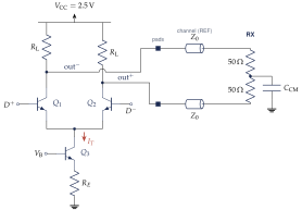
The Open-SERDES driver (Figure 9.5) is Figure 9.4(c) in differential form. An HBT pair \(Q_1/Q_2\) steers the tail current \(I_T\) into one of two loads \(R_\mathrm{L}=Z_0=50\,\Omega\), which are also the TX back-terminations. The RX terminates the line in 100 Ω differential.
Swing
When \(Q_2\) takes all of \(I_T\), the current divides between its own load and the line, so each output sees \(R_\mathrm{L}\parallel Z_0=25\,\Omega\) and swings \(I_T\cdot25\,\Omega\) single-ended. The differential voltage flips sign with the data, so \(V_{d,\mathrm{pp}}=2\cdot I_T\cdot25\,\Omega =I_TZ_0\).
Voltage mode
The alternative is a voltage-mode (VM) driver, usually a source-series-terminated (SST) one: each output is an inverter-like switch pair in series with a resistor, \(R_\mathrm{on}+R_S=Z_0\) [25]. Its current flows only around the loop of TX resistor, line, 100 Ω RX termination, line and TX resistor: \(4Z_0=200\,\Omega\). A supply \(V_s\) drives \(I=V_s/4Z_0\), the RX sees \(\pm V_s/2\), and \(V_{d,\mathrm{pp}}=V_s\).
Key equation · Driver current for a differential swing \(V_{d,\mathrm{pp}}\)
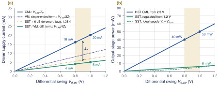
\[I_\mathrm{CML}=\frac{V_{d,\mathrm{pp}}}{Z_0},\qquad I_\mathrm{VM,\,SE\ term.}=\frac{V_{d,\mathrm{pp}}}{2Z_0},\qquad I_\mathrm{VM,\,diff.\ term.}=\frac{V_{d,\mathrm{pp}}}{4Z_0}. \tag{9.3}\] CML needs four times the current of VM into a differential termination: half of it flows in its own termination, and it never reverses through the line.
Worked Example 9.2 · CML versus SST at Open-SERDES swings
CML: 800 mVppd needs \(I_T=0.8/50=16\,\mathrm{mA}\), 40 mW from 2.5 V. At 1 Vppd (the model value, \(A=0.5\,\mathrm{V}\)) it needs 20 mA and 50 mW. The output common mode sits \(I_T\times25\,\Omega =0.5\,\mathrm{V}\) below \(V_\mathrm{CC}\), and each output moves between 1.75 and 2.25 V.
SST: 800 mVppd needs \(I=0.8/200=4\,\mathrm{mA}\) from \(V_s\approx0.8\,\mathrm{V}\): 3.2 mW, or 4.8 mW through a regulator from 1.2 V (6 mW at 1 Vppd). Keep \(R_\mathrm{on}\le10\,\Omega\), so a \(\pm30\,\%\) spread moves the output impedance by only \(\pm3\,\Omega\).
Verdict: SST saves about 44 mW (Figure 9.6), but Open-SERDES uses CML: a passive-resistor impedance with no calibration loop, constant supply current, FFE taps that leave the impedance untouched, and fast HBTs instead of CMOS pre-drivers passing 200 ps (4.8 FO4) pulses. SST is the power upgrade for a second tape-out.
Why HBTs
A CML stage must switch its tail current fully. A bipolar pair splits it as \(\Delta I=I_T\tanh(V_\mathrm{id}/2V_T)\), so \(V_\mathrm{id}\approx4V_T\approx100\,\mathrm{mV}\) steers 96 % of it at any current. A MOS pair needs \(\sqrt2\,V_\mathrm{OD}\), typically 200–300 mV. The HBT’s \(g_\mathrm{m}/I_C=1/V_T=38.7\,1/\mathrm{V}\) is also several times a MOSFET’s.
Worked Example 9.3 · HBT versus MOS in a 2.5 GHz CML stage
Given: a mux or pre-driver stage loaded by \(C_\mathrm{L}=40\,\mathrm{fF}\), with \(f_\mathrm{3dB}\ge7.5\,\mathrm{GHz}\), so \(\tau\le21\,\mathrm{ps}\). By Equation (9.2), \(R_\mathrm{L}=500\,\Omega\) gives \(\tau=20\,\mathrm{ps}\); \(\Delta V=300\,\mathrm{mV}\) then needs \(I_T=0.6\,\mathrm{mA}\), or 1.5 mW from 2.5 V.
HBT pair: at the crossing each device carries 0.3 mA, \(g_\mathrm{m}=11.6\,\mathrm{mS}\), and the gain is \(g_\mathrm{m}R_\mathrm{L}=\Delta V/2V_T=\mathbf{5.8}\). Full switching needs about 104 mV.
MOS pair at the same current with \(V_\mathrm{OD}=150\,\mathrm{mV}\): \(g_\mathrm{m}=4\,\mathrm{mS}\), gain \(\Delta V/V_\mathrm{OD}=\mathbf{2}\), full switching at 212 mV. More gain needs wider devices, more \(C_\mathrm{L}\) and more current. A chain of HBT stages can therefore run at smaller swing, with fewer and smaller stages.
Headroom and the \(\mathrm{BV}_\mathrm{CEO}\) limit
SG13G2 HBTs break down at about \(\mathrm{BV}_\mathrm{CEO}\approx1.6\,\mathrm{V}\) (check the PDK). On 2.5 V the off driver transistor is at risk: its collector sits at the high output level. Stack up Worked Example 9.2 at 1 Vppd. Outputs: 2.25 V (off) and 1.75 V (on). Bases high: 1.9 V, from a pre-driver whose common-mode resistor pulls its outputs 0.6 V below \(V_\mathrm{CC}\). Common emitter: \(1.9-V_\mathrm{BE}\approx1.0\,\mathrm{V}\). So \(V_\mathrm{CE}=0.75\) V on and 1.25 V off, with 1.0 V left for the tail. The 0.35 V margin is eaten by \(V_\mathrm{CC}+5\,\%\), overshoot and reflections; an emitter-follower pre-driver with bases near 1.6 V would leave the off device at 1.5 V nominal. Check every \(V_\mathrm{CE}\) at every corner with the real RX termination attached: a far end terminated to ground moves the output common mode.
9.5The FFE inside the driver
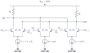
Chapter 6 chose the taps; here we build them. Put one differential pair per tap on the same pair of loads, drive each with its own copy of the data, and set each tail current to the tap weight (Figure 9.7). The loads add the currents, which forms the FIR sum of Section 6.2. Negative side taps cost nothing: swapping a pair’s base inputs inverts its contribution.
Key equation · Current-summing FFE
\[v_{d}[n]=\frac{Z_0}{2}\,I_T\sum_{k=-1}^{1}c_k\,a_{n-k},\qquad c_k=\pm\frac{I_k}{I_T},\qquad \sum_k\lvert c_k\rvert=\frac{I_{-1}+I_0+I_1}{I_T}=1 . \tag{9.4}\] The peak-swing constraint of Section 6.2 holds by construction: the taps are slices of one fixed tail current.
Making the delayed copies
No 5 GHz clock is needed. Call the half-rate streams \(E_m\) (bit \(2m\)) and \(O_m\) (bit \(2m+1\)). The main mux selects \((E_m,O_m)\). The post-tap mux must emit bit \(2m-1\) in the even slot and bit \(2m\) in the odd slot, so it selects \((O_{m-1},E_m)\); the pre-tap mux selects \((O_m,E_{m+1})\). About four extra latches on the 2.5 GHz clock keep these inputs glitch-free (Figure 9.3b).
Worked Example 9.4 · Tap currents for the \(-6\) dB preset
The de-emphasis of a 2-tap setting is \(\mathrm{DE}=20\log_{10}\big[(\lvert c_0\rvert+\lvert c_1\rvert)/(\lvert c_0\rvert-\lvert c_1\rvert)\big]\), the ratio of transition to repeated-bit swing. For 6 dB that ratio is 2; with \(\lvert c_0\rvert+\lvert c_1\rvert=1\), \(\lvert c_0\rvert-\lvert c_1\rvert=0.5\), so \(c_0=0.75\) and \(c_1=-0.25\), the PCIe preset of Section 6.2. (The often-quoted \(c_1=-1/3\) is the 9.5 dB setting.)
At 1 Vppd (\(I_T=20\,\mathrm{mA}\)): \(I_0=15\,\mathrm{mA}\), \(I_1=5\,\mathrm{mA}\). Transition bits swing \((15+5)\,\mathrm{mA}\times Z_0=1.0\,\mathrm{V}_\mathrm{ppd}\), repeated bits \((15-5)\times50=0.5\,\mathrm{V}_\mathrm{ppd}\). The supply stays at 50 mW for every preset.
Resolution: build \(I_T\) from 32 cells of 0.625 mA (5 bits). The \(-6\) dB preset is exact (24 and 8 cells). The \(-3.5\) dB preset needs 5.3 cells; five give \(c_1=-0.156\) and 3.2 dB, which is harmless because the eye is flat near its optimum (Chapter 6). A pre-tap moves in steps of \(1/32=0.031\).
The resolution trade-off
Range and resolution cost capacitance, not current. Sizing each pair for its largest current (20 mA main, 8 mA for \(\lvert c_1\rvert\le0.4\), 3 mA for \(\lvert c_{-1}\rvert\le0.15\)) loads the output with 31 mA worth of collectors, 1.55 times a plain driver. A segmented driver instead uses 32 identical cells, each with a selector in its pre-driver that assigns it to the pre, main or post stream: the output always sees exactly 20 mA of devices, and the cost moves into the pre-drivers.
What this means for your design
Build the FFE from current. The tail current is fixed, so power and output impedance do not depend on the preset, and \(\sum\lvert c_k\rvert=1\) holds automatically. Five bits are enough. Spend layout effort on matching the three tap paths: a 10 ps skew between \(D_n\) and \(D_{n-1}\) moves the de-emphasis edge by 0.05 UI.
9.6Pad, ESD and bandwidth
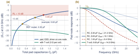
At the pad the driver’s collector capacitance, the termination’s parasitics, the ESD diodes and the bond pad hang on one node (Figure 9.9a). That node sees \(R_\mathrm{L}\parallel Z_0=25\,\Omega\), so the total capacitance \(C_p\) makes a pole at \[f_\mathrm{3dB}=\frac{1}{2\pi(Z_0/2)C_p}=\frac{1}{\pi Z_0C_p} \tag{9.5}\] and spoils the return loss (Section 3.4). The ESD protection cannot be left out: dual diodes from the pad to both rails, plus a supply clamp, steer an electrostatic discharge away from the HBT and thin-oxide junctions. Diodes rated for a few kilovolts of human-body-model discharge are large and often dominate \(C_p\).
Worked Example 9.5 · The Open-SERDES pad capacitance budget
Illustrative values (extract the real ones from layout): bond pad 80 fF, ESD diodes 250 fF, driver collectors and termination parasitics 300 fF: \(C_p=0.63\,\mathrm{pF}\).
Return loss at \(f_\mathrm{N}\): \(x=\omega Z_0C_p=0.495\) and \(\lvert S_{11}\rvert=x/\sqrt{4+x^2}=0.24\), or \(-12.4\) dB. It passes a 10 dB target (\(C_p\le0.85\,\mathrm{pF}\)) but fails 15 dB (\(C_p\le0.46\,\mathrm{pF}\)). Bandwidth: \(f_\mathrm{3dB}=1/(\pi\cdot50\cdot0.63\,\mathrm{pF})=10.1\,\mathrm{GHz}\), four times \(f_\mathrm{N}\).
System check: the REF model assumes 300 fF per pad. With c_pad=0.63e-12 in channel() the loss at \(f_\mathrm{N}\) grows from 17.4 to 17.8 dB and the FFE-only PDA eye drops from 62 to 54 mV. Always rerun the system model with the extracted pad capacitance.
The T-coil
When the budget does not close, a bridged T-coil separates the capacitance from the line [26, 27]. Two coupled inductors connect pad and termination, the capacitive load hangs on their center tap, and a small \(C_B\) bridges the ends (Figure 9.9b). With the right values the inductive and capacitive impedances cancel exactly [28].
Key equation · Bridged T-coil, \(\zeta=1/\sqrt2\)
\[L_1=L_2=\frac{R^2C}{2(1+k)},\quad k=\frac{4\zeta^2-1}{4\zeta^2+1}=\frac13,\quad C_B=\frac{C}{16\zeta^2}=\frac{C}{8},\quad Z_\mathrm{in}=R\ \text{at all }f. \tag{9.6}\] The total inductance is \(L_1+L_2+2M=R^2C\). From a current source, the capacitor node then has 2.83 times the bandwidth of the plain \(RC\). In a doubly terminated pad the plain pole already sees \(R/2\), so the bandwidth gain is \(\sqrt2\); the bigger gain is in return loss.
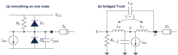
For \(C=0.63\,\mathrm{pF}\) and \(R=50\,\Omega\), Equation (9.6) gives \(L_1=L_2=0.59\,\mathrm{nH}\), \(M=0.20\,\mathrm{nH}\) and \(C_B=79\,\mathrm{fF}\) (often the coil’s own inter-winding capacitance): better than 25 dB of return loss at \(f_\mathrm{N}\) with 3 Ω per coil (Figure 9.8). In SG13G2 it fits in roughly \(60\,\mu\mathrm{m}\times60\,\mu\mathrm{m}\) on the thick top metals; take \(k\), \(C_B\) and self-resonance from EM simulation (Section 15.4).
Design rule of thumb
At 5 Gb/s a T-coil is optional. Below about 0.85 pF the pad already meets 10 dB of return loss at \(f_\mathrm{N}\), and its pole at 7.5 GHz or above costs little ISI. Add a T-coil if ESD and driver push \(C_p\) toward 1 pF, or if the return-loss target is tighter (15 dB at \(f_\mathrm{N}\)). Either way, give the system model your extracted \(C_p\), not the 300 fF of REF.
9.7TX design checklist
Table 9.1 collects the checks and a first-cut power estimate of about 100 mW, half of it in the driver (Section 14.6 adds the RX and clocking).
| Block | Check before layout | Power |
|---|---|---|
| 3-tap CML driver | \(I_T=20\) mA (16 mA at 0.8 Vppd); every \(V_\mathrm{CE}<\mathrm{BV}_\mathrm{CEO}\) at \(V_\mathrm{CC}+5\,\%\) | 50 mW |
| Pre-drivers (\(\times3\)) | full switching (\(\ge4V_T\)); tap paths matched to a few ps | 10 mW |
| 2:1 muxes (\(\times3\)), latches (\(\times4\)) | glitch-free phases; 5-bit tap DACs, \(-3.5\)/\(-6\) dB presets | 21 mW |
| Clock buffers, 4:2, \(\div2\) | duty cycle \(50\pm1\,\%\); clock-to-data windows at all corners | 20 mW |
| CMOS 16:4 (1.2 V) | FO4 measured; timing closed at 625 MHz | 3 mW |
| Termination and pad | poly \(R_\mathrm{L}\) for 20 mA; \(C_p<0.85\) pF or T-coil; RL \(\ge10\) dB at \(f_\mathrm{N}\) | – |
| Total TX | 41 mA from 2.5 V, 2.5 mA from 1.2 V | \(\approx\)104 mW |
Key takeaways
A CMOS clock tree needs 8 FO4 per period. With \(t_\mathrm{FO4}\approx42\) ps (55 ps slow), full-rate CMOS cannot reach 5 Gb/s and half-rate CMOS fails at the slow corner, so the final 2:1 mux and its 2.5 GHz clock are HBT CML.
A half-rate mux uses the clock as the select. Each input must change only while deselected, and the clock duty cycle becomes the UI width.
Double termination absorbs echoes at both ends for half the swing. A CML driver needs \(I_T=V_{d,\mathrm{pp}}/Z_0\): 20 mA and 50 mW from 2.5 V at 1 Vppd, four times a voltage-mode driver.
HBTs switch fully with about 100 mV: a 2.5 GHz CML stage has a gain of 5.8 against 2 for MOS at the same current.
The off driver transistor sees the highest \(V_\mathrm{CE}\); keep it below \(\mathrm{BV}_\mathrm{CEO}\approx1.6\) V at every corner.
The FFE is current-steering pairs on shared loads; \(-6\) dB is \(c_0=0.75\), \(c_1=-0.25\) (15 and 5 mA). Five bits are enough.
Keep \(C_p\) below 0.85 pF for 10 dB return loss at \(f_\mathrm{N}\); a T-coil (\(k=1/3\), \(C_B=C/8\)) absorbs larger loads.
Generated from book/tutorial/chapters/09_tx.tex. Figure, table and equation numbers match the PDF edition.