Chapter 15Design and Verification Flow with Open Tools
From a Python model to a GDS file and a test bench, with nothing but open-source tools: which tool does what, how the model and the circuits keep each other honest, and how to prove the chip works.
In this chapter you will learn
Name the open tool used at each stage of the Open-SERDES flow and say what it checks.
Close the loop between the serdespy model and the transistor-level circuits by back-annotating simulated responses.
Choose a testbench, a measurement and a pass/fail criterion for every block, including corners and Monte Carlo.
Apply the layout rules that matter at 5 Gb/s: symmetry, current density, metal width, inductors, extraction and decoupling.
Plan the lab bring-up: test board, loopback, on-chip PRBS checking and the measurements that compare silicon with the model.
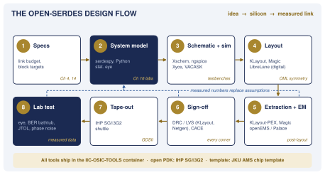
The flow in Figure 15.1 runs left to right, but it is not a pipeline. Every stage feeds numbers back to the system model, and the chip is ready for tape-out only when the model, rerun with those numbers, still shows margin at every corner.
15.1The open toolchain
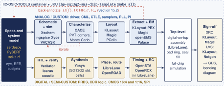
Every tool in this chapter ships in one Docker image, IIC-OSIC-TOOLS [2], together with the IHP SG13G2 PDK [1]; pinning one image tag gives the whole team identical tools. The Open-SERDES repository builds on the JKU analog mixed-signal chip template [5] (it needs image 2026.06 or later). Its recursive Makefiles make one make all run every testbench including PVT and Monte Carlo, run DRC, LVS and extraction on the analog macros, harden the digital logic and assemble the chip digital-on-top with seal ring, pad frame and fill, run a full-chip LVS without black boxes, and draw the bonding diagram. GitHub Actions rerun it on every commit, so a broken block is noticed the day it breaks.
Figure 15.2 maps the tools onto the flow, and Table 15.1 says what each one is for.
| Tool | Purpose in Open-SERDES | Stage |
|---|---|---|
| serdespy [3], PyBERT [44] | link models, eyes, BER (Chapter 16); PyBERT adds a GUI and IBIS-AMI | system model |
| scikit-rf [18] | Touchstone files, mixed-mode S-parameters, de-embedding | model, EM, lab |
| Xschem [45] | schematics, symbols, testbench netlists for every simulator | schematic |
| ngspice [46] | .op, .ac, .noise, .tran, transient noise, Verilog-A via OSDI |
simulation |
| Xyce [47], VACASK [48] | parallel SPICE for large post-layout runs; Verilog-A simulator with PSS and HB | simulation |
| CACE [49] | YAML datasheet: runs testbenches over corners, checks min/typ/max limits | characterization |
| KLayout [50], Magic [51] | layout editing; IHP DRC and LVS decks; RC extraction (Magic) | layout, sign-off |
| Netgen [52], KLayout-PEX [53] | LVS comparison; parasitic extraction for SG13G2 | sign-off, extraction |
| openEMS [54], Palace [55] | FDTD and FEM field solvers for inductors, pads and package | EM |
| Verilator [56], Icarus [57], cocotb [58] | Verilog simulation and lint; Python testbenches for PRBS, CDR, SPI | RTL |
| Yosys [59], LibreLane [60] | synthesis to SG13G2 cells; RTL-to-GDS flow (successor of OpenLane 2 [61]) | digital |
| OpenROAD [62], OpenSTA [63] | placement, clock tree, routing; static timing (inside LibreLane) | digital |
15.2The model–circuit loop
The labs of Chapter 16 describe each block by an ideal transfer function. The circuits will not match those ideals, and the only way to know whether the difference matters is to put the circuit’s real response back into the model (Figure 15.3). Because the link is linear up to the sampler, each simulated block becomes one more factor in the cascade:
Key equation · Back-annotating the link model
\[H_\mathrm{link}(f) = H_\mathrm{TX}(f)\,H_\mathrm{ch}(f)\,H_\mathrm{CTLE,ckt}(f),\qquad p_\mathrm{TX}(t) = s(t) - s(t-T_\mathrm{b}),\qquad \sigma_\mathrm{n}^2 = \sum_i \sigma_{n,i}^2 . \tag{15.1}\]
Here \(s(t)\) is the simulated step response of the driver into its load, so \(p_\mathrm{TX}(t)\) is its real 1-UI pulse, with finite edges and any ringing; sampling it at \(T_\mathrm{b}\) spacing gives the effective FIR taps. The CTLE enters through its .ac response, and each noise source through its rms value from .noise or Monte Carlo.
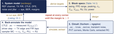
Listing 15.1 loads an ngspice AC sweep into the Lab 4 model. In ngspice, wrdata ctle_ac.txt v(outp,outn) after an ac dec 100 1meg 100g writes frequency, real and imaginary parts in three columns. The sweep is resampled onto the model’s 10 MHz grid, the end values are held outside it, and the DC point is forced real, as sdp.freq2impulse requires.
from common import *                        # F grid, channel(), impulse(), ...
f_sp, re, im = np.loadtxt("ctle_ac.txt", usecols=(0, 1, 2), unpack=True)
H_sp = re + 1j * im                         # wrdata ctle_ac.txt v(outp,outn)
mag = np.interp(F, f_sp, np.abs(H_sp))      # resample onto the model grid;
phs = np.interp(F, f_sp, np.unwrap(np.angle(H_sp)))  # holds end values
H_ckt = mag * np.exp(1j * phs)
H_ckt[0] = mag[0]                           # DC must be real
h_link, t = impulse(channel() * H_ckt)      # REF x circuit CTLE
bits = np.tile(sdp.prbs7(1), 40)
y = through(tx_wave(bits), h_link)
report_eye("REF + ngspice CTLE", y, bits)
Worked Example 15.1 · What a slow second pole costs
Check: feed Listing 15.1 the ideal ctle(8) response sampled from 1 MHz to 100 GHz. It returns 60.0 mV and 0.56 UI, exactly the Lab 5 pre-DFE eye, so the resampling loses nothing.
A realistic circuit: suppose the extracted CTLE has its output pole at \(f_{p2}=6\) GHz instead of the 10 GHz of the model, because the four samplers load it more than planned. The 12 dB eye drops from 104.0 to 98.0 mV and the 14 dB eye from 113.3 to 107.4 mV, about 6 %. At 5 GHz the loss is 9 %. That is affordable against 76 mV of margin, but it is exactly the kind of number that only the loop reveals.
15.3Testbenches
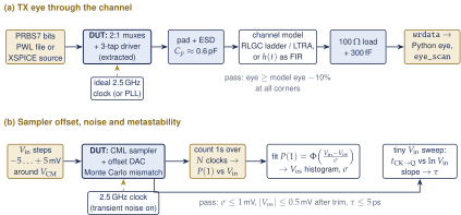
Every specification in Table 14.2 needs a testbench that measures it and a pass/fail limit. Table 15.2 lists the key ones and Figure 15.4 sketches two of them.
| Block | Testbench | Measure | Pass |
|---|---|---|---|
| TX serializer + driver | .tran, PRBS7 into 100 Ω + \(C_p\); then through the channel model |
swing, edges, DCD, eye, every \(V_\mathrm{CE}\) | 0.8–1.0 Vppd; DCD + DDJ \(\le8\) ps; \(V_\mathrm{CE}<\mathrm{BV}_\mathrm{CEO}\) |
| Termination, pad | .ac or .sp with ESD and pad parasitics |
\(S_{11}\), \(C_p\) | RL \(\ge10\) dB at 2.5 GHz |
| CTLE | .ac at every code; .noise; large-signal .tran |
peaking, \(f_z\), \(f_{p2}\), noise, linearity | 0–12 dB; \(f_{p2}\ge7.5\) GHz; \(\le0.25\) mV |
| DFE summer | .tran with tap 1 toggling every UI |
settling inside the tap-1 loop | \(t_\mathrm{CK\to Q}+t_\mathrm{settle}+t_\mathrm{setup}\le\) 1 UI |
| Sampler | DC-step sweep counting \(P(1)\), Monte Carlo; tiny-input sweep; transient noise | \(V_\mathrm{os}\), \(\sigma\), \(\tau\) | \(\sigma\le1\) mV, \(\tau\le5\) ps, trim range \(\ge\pm3\sigma\) |
| PLL | lock transient; VCO phase noise (transient noise, or PSS/pnoise in VACASK); Python loop model | lock time, \(\mathcal{L}(f)\), RJ | RJ \(\le1\) ps rms |
| PPF + PI | .tran at all 64 codes |
phase vs. code, amplitude | I/Q \(\le2^{\circ}\), INL \(\le1^{\circ}\) |
| CDR logic | cocotb with a Python phase model driving the early/late inputs | lock, ppm range, dither | \(\pm300\) ppm; \(\le20\) ps pp |
| PRBS, SPI | cocotb on Verilator or Icarus; error injection | error count, resync | exact counts |
The channel in SPICE
The REF channel has skin-effect loss that grows as \(\sqrt f\) and dielectric loss that grows as \(f\) (Section 3.3). Neither open simulator models that directly in a transient. ngspice offers the lossless line (T), the SPICE3 lossy line LTRA (O), and the single and coupled lossy lines TXL and CPL; all of them take constant per-unit-length \(R\), \(L\), \(G\), \(C\). It has no HSPICE-style W-element with frequency-dependent tables and no element that reads a Touchstone file; its .sp analysis computes S-parameters of a circuit, it does not import them. Xyce has TRA, LTRA and a lumped line (YTRANSLINE), and a linear YLIN device that reads Touchstone data, documented mainly for harmonic-balance and other frequency-domain analyses. So there are three practical options: (i) a long ladder of RLGC sections, (ii) a behavioral source that convolves with \(h(t)\), or (iii) splitting the problem at the channel.
Key equation · Sections needed for a lumped line model
\[\Delta\ell\le\frac{\lambda_\mathrm{min}}{10}=\frac{v}{10\,f_\mathrm{max}} \quad\Rightarrow\quad N\ge\frac{10\,\ell\,f_\mathrm{max}}{v} \tag{15.2}\]
For REF, \(\ell=1\) m, \(v=c/\sqrt{4}=1.5\times10^8\) m/s and \(f_\mathrm{max}=10\) GHz give \(N\ge667\) sections, each needing extra R–L branches to mimic the skin effect. That is slow and hard to fit. Option (iii) is exact for a matched link and is what Open-SERDES uses: simulate the TX into a 50 Ω-per-side load in SPICE, export the differential waveform, apply the channel in Python with through(x, h), and feed the result back into the RX testbench as a PWL source behind 50 Ω per side.
Corners, Monte Carlo and CACE
The SG13G2 model libraries have typical, best-case and worst-case sections for MOS devices, HBTs and resistors; combine them with supply \(\pm5\) % and 0–85 \(^\circ\)C. Mismatch-sensitive specs (sampler offset, I/Q phase, mirror ratios) need Monte Carlo, and the number of runs sets how well you know the answer.
Key equation · How many Monte Carlo runs
\[\frac{\Delta\hat\sigma}{\sigma}\approx\frac{1}{\sqrt{2N}} \tag{15.3}\]
Fifty runs know \(\sigma\) to about 10 %, 200 runs to 5 % (for the sampler, \(4.9\pm0.25\) mV). CACE turns all of this into a datasheet: a YAML file per block lists each parameter with its minimum, typical and maximum limits, the testbench that measures it and the conditions to sweep; CACE runs every combination and reports pass or fail, so Table 14.2 becomes an executable checklist.
15.4Layout for high speed
At 5 Gb/s a layout can lose the margin that the schematic won. Six habits keep it.
Symmetry
Draw every differential circuit as two mirror-image halves and route each pair as a pair. Place HBT pairs and mirror devices common-centroid (ABBA) with dummies at the ends. A 10 ps skew between FFE tap paths moves the de-emphasis edge by 0.05 UI (Section 9.5); 1 % of clock duty-cycle error costs 4 ps (Section 12.5).
Current density
An HBT reaches its peak \(f_T\) at one collector current density. Size each emitter so that the switching transistors sit near that point at their tail current, from the npn13G2 \(f_T\)-versus-\(J_C\) curves of the PDK; past the peak, \(f_T\) collapses.
Metal width
Every DC path needs \(w\ge I/J_\mathrm{max}\), with the electromigration limit \(J_\mathrm{max}\) of that layer and temperature from the SG13G2 rules. Route the 20 mA driver tail, its loads and the 2.5 V straps on TopMetal1 and TopMetal2; a few ohms of strap under 77 mA of CML current shift every common-mode level in the chip.
Inductors and EM
Put the 4 nH VCO inductor (and any T-coil) on TopMetal2, away from other metal. IHP’s gds2openEMS and gds2palace scripts take the GDS and a stackup file, run openEMS (FDTD) or Palace (FEM), and return S-parameters for a \(\pi\)-model or a wideband fit [1]. Match \(L\) and \(Q\) to the team’s measured inductor before trusting the flow.
Extraction and isolation
Extract every analog block with KLayout-PEX or Magic and resimulate; clock-to-data coupling and the wiring capacitance on the CTLE output are the usual surprises. Surround the CML blocks, the VCO and the samplers with substrate guard rings, away from the switching CMOS logic.
Decoupling
CML draws constant current; CMOS draws its charge in spikes at the clock edges, and that charge must come from on-chip capacitors.
Worked Example 15.2 · Decoupling the deserializer
Switched capacitance: the 1:16 deserializer burns 5 mW at 1.2 V and 312.5 MHz, so \(\alpha C_\mathrm{sw}=P/(V_\mathrm{DD}^2f)=5\,\mathrm{mW}/(1.44\times312.5\,\mathrm{MHz})=11\,\mathrm{pF}\) is switched every cycle.
Worst case: if all of it switches on one edge, before the package can refill the rail, the droop is \(\Delta V/V\approx C_\mathrm{sw}/(C_\mathrm{sw}+C_\mathrm{dec})\). For 5 % droop, \(C_\mathrm{dec}\ge19\,C_\mathrm{sw}=210\,\mathrm{pF}\): about 0.14 mm\(^2\) of MIM capacitor at roughly 1.5 fF/m\(^2\) (check the PDK value). Inside the synthesized digital macros, LibreLane adds decap cells [5]; budget the rest as MIM next to the macro, and count it in the die area.
The digital flow
The PRBS logic, the CDR loop filter, the SPI registers and the slow CMOS serializer and deserializer stages are Verilog, verified with cocotb and hardened by LibreLane. Synthesize what runs at 625 MHz or slower; place the 1.25 GHz deserializer stage and the CMOS-to-CML converters by hand from standard cells.
Sign-off
DRC with the IHP KLayout decks (Magic as a second opinion), LVS with KLayout or Netgen, then antenna and density checks after fill, and the template’s full-chip LVS without black boxes [5]: run it whenever a macro changes.
15.4.1Repository structure
The Open-SERDES repository keeps the recursive layout of the JKU template: every analog block is a macro with its own schematics, testbenches, layout, verification and Makefile, so a block can be built, simulated and verified alone. The listing shows these folders for tx_serializer; every other macro has the same ones. The digital half (PRBS, the CMOS serializer and deserializer stages, the CDR loop filter and SPI) is not a macro: it lives in rtl/ and is hardened with the chip, digital-on-top. Open-SERDES adds four folders of its own: spec/, the one specification file that the link model and every testbench read; model/; channels/; and lab/, for the test board and the measured data of Section 15.5. The others (flow/, layout/, netlist/, ip/, packaging/, release/ and doc/) come with the template.
open-serdes/                  # from ihp-sg13g2-ams-chip-template
|-- Makefile                  # make model && make all
|-- spec/                     # one spec file: model and testbenches
|-- model/                    # link model, stat. eye, GUI, labs (Ch. 16)
|-- channels/                 # S-parameters: REF, REF-10, 802.3, boards
|-- macros/                   # analog macros, one per block
|   |-- tx_serializer/        # CML 4:2 and 2:1, CMOS-to-CML
|   |   |-- schematic/  testbenches/  layout/  netlist/
|   |   |-- verification/     # drc/  lvs/  cace/ (limits from spec/)
|   |   |-- scripts/
|   |   |-- final/            # GDS, LEF, lib for the chip assembly
|   |   `-- Makefile          # make all: build, sim, DRC, LVS
|   |-- tx_ffe_driver/        # 3-tap CML driver, termination, ESD, pad
|   |-- rx_ctle/              # termination, ESD, loopback mux, CTLE
|   |-- rx_sampler_dfe/       # 2-tap DFE summer, four samplers
|   |-- pll_lcvco/            # integer-N PLL, LC VCO, dividers
|   |-- cdr_pi/               # I/Q generation, two phase interpolators
|   `-- cml_lib/              # shared HBT CML cells
|-- rtl/                      # PRBS, CMOS SER/DES, CDR loop filter, SPI
|-- flow/                     # LibreLane: rtl/ hardened digital-on-top
|-- verification/             # link regression, eye checks, full-chip DRC/LVS
|-- layout/  netlist/  ip/  packaging/  release/
|-- lab/                      # test board, bring-up scripts, data
`-- doc/                      # documentation (from the template)
The template’s make macro FROM=inverter NAME=rx_ctle creates a new macro from its example. The macro’s CACE datasheet reads every limit from spec/, so a number changes in one place only.
15.5Testing the chip in the lab
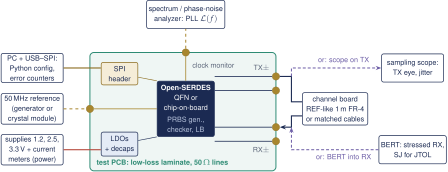
Figure 15.5 shows the bring-up bench. The test board carries the chip, SMA connectors for TX\(\pm\), RX\(\pm\), the reference clock and a divided clock-monitor output, local regulators and decoupling, and an SPI header. Keep the 50 Ω traces from the pads to the SMAs short and identical within each pair, and de-embed them with scikit-rf from a measured test structure.
Bring-up order
(1) Supplies and currents against Table 14.3. (2) SPI read-back of every register. (3) PLL lock, seen on the clock monitor. (4) TX eye with PRBS7 on a scope. (5) Near-end loopback with the on-chip checker: this tests the chip without the board. (6) The external loop through the channel board, sweeping FFE presets and CTLE codes. (7) Freeze the CDR, step the PI code through the override register and count errors at each step: an on-chip bathtub, with the offset DACs giving the vertical scan.
Key equation · Bits needed to claim a BER
\[N_\mathrm{bits}\ge\frac{-\ln(1-\mathrm{CL})}{\mathrm{BER}}\approx\frac{3}{\mathrm{BER}}\quad\text{(zero errors, CL = 95\,\%)} \tag{15.4}\]
Claiming \(10^{-12}\) at 95 % confidence takes \(3\times10^{12}\) error-free bits, or 600 s at 5 Gb/s: ten minutes per setting, which is why the checker is on chip.
| Measurement | Setup | Target or comparison |
|---|---|---|
| TX eye and jitter | PRBS7, sampling scope at the TX SMAs | 0.8–1.0 Vppd; edges, DCD vs. simulation |
| BER and bathtub | loopback or channel board; on-chip checker; PI-code sweep | BER \(\le10^{-12}\) (10 min); bathtub vs. Lab 6 |
| Equalizer sweep | FFE presets \(\times\) CTLE codes \(\times\) DFE on/off | best setting vs. Section 8.5 |
| Jitter tolerance | BERT with sinusoidal jitter into RX | above the mask of Section 13.5 |
| PLL phase noise | clock monitor into a phase-noise analyzer | \(\mathcal{L}(1\,\mathrm{MHz})\); RJ \(\le1\) ps rms |
| Return loss | VNA at the RX SMAs, de-embedded | RL \(\ge10\) dB at 2.5 GHz |
| Power | current per supply rail in each mode | vs. Table 14.3 |
Table 15.3 is the measurement plan. Each row ends in a comparison with a model number, which closes the last loop of the flow: when silicon and model disagree, the model is updated first, and the next design starts from it.
Key takeaways
One container, IIC-OSIC-TOOLS, holds every tool and the SG13G2 PDK; the JKU template turns the whole flow into
make allwith regression on every commit.The system model is not finished when the circuits start: back-annotate the CTLE
.acresponse, the driver step and the noise and offset of every block, and rerun the eye at each corner.Open SPICE engines have only constant-RLGC lossy lines; for REF, simulate the TX into a matched load and apply the channel in Python.
Run every analog testbench at PVT corners; \(N\) Monte Carlo runs know \(\sigma\) to \(1/\sqrt{2N}\); let CACE check every limit of the specification table.
Layout for 5 Gb/s means mirror symmetry, HBTs at their peak-\(f_T\) current density, metal sized for the DC current, EM-simulated inductors on TopMetal2, extraction, guard rings and real decoupling area.
The chip tests itself: PRBS generator, checker and loopback verify \(10^{-12}\) in ten minutes; instruments confirm the eye, jitter tolerance, phase noise and power against the model.
Generated from book/tutorial/chapters/15_flow.tex. Figure, table and equation numbers match the PDF edition.