Chapter 3The Channel
Copper is not a wire at 5 Gb/s: it is a lossy, reflective transmission line, and its pulse response sets almost every number in the rest of this book.
In this chapter you will learn
Decide when a trace is a transmission line, and compute \(Z_0\) and the delay from its RLGC parameters.
Explain why conductor loss grows as \(\sqrt f\) and dielectric loss as \(f\), and estimate FR-4 loss in dB per inch.
Predict reflections from terminations, pads, bondwires and via stubs, and read them in a TDR plot.
Use S-parameters, including the mixed-mode \(S_{dd21}\) of a differential pair.
Turn \(S_{21}(f)\) into a causal impulse response and a pulse response.
Know the Open-SERDES reference channel REF and its cursors.
3.1What is the channel?
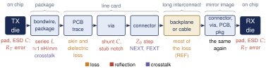
The channel is everything between the transmitter’s output transistors and the receiver’s input transistors. Figure 3.1 follows a bit across a typical board-to-board link. Long traces and cables attenuate high frequencies (loss). Short lumps such as bondwires, pads and vias change the impedance and send part of the wave back (reflections). Dense pins and connectors couple neighboring lanes (crosstalk). We treat each mechanism in turn and then combine them into one transfer function \(H_\mathrm{ch}(f)\) and one pulse response \(p(t)\), the two objects that the link-analysis tools of Chapter 4 work with.
3.2Transmission lines
3.2.1When is a wire a transmission line?
A wire is lumped when its voltage is the same everywhere at any instant. It becomes a transmission line when the signal changes noticeably while the wave travels along it. The usual rule compares the one-way delay \(t_d\) with the rise time \(t_r\) [15, 16]: \[t_d \gtrsim \frac{t_r}{6} \quad\Longleftrightarrow\quad \ell \gtrsim \frac{t_r\, v}{6}, \tag{3.1}\] where \(v\) is the propagation velocity. Equivalently, a line longer than about a tenth of a wavelength at the highest frequency of interest is a transmission line.
3.2.2The telegrapher model
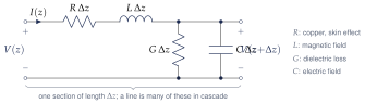
A transmission line is a ladder of tiny identical sections (Figure 3.2). Each section of length \(\Delta z\) has a series resistance \(R\,\Delta z\) (the copper), a series inductance \(L\,\Delta z\) (the magnetic field around the current), a shunt capacitance \(C\,\Delta z\) (the electric field to the return plane) and a shunt conductance \(G\,\Delta z\) (leakage through the dielectric). KVL and KCL around one section, in the limit \(\Delta z\to0\), give the telegrapher equations \[\frac{\partial V}{\partial z} = -(R + j\omega L)\, I, \qquad \frac{\partial I}{\partial z} = -(G + j\omega C)\, V .\] Eliminating \(I\) gives \(\partial^2 V/\partial z^2 = \gamma^2 V\), whose solution is a forward and a backward wave, \(V(z) = V^+e^{-\gamma z} + V^-e^{+\gamma z}\).
Key equation · Propagation constant, impedance and velocity
\[\begin{gathered} \gamma = \alpha + j\beta = \sqrt{(R + j\omega L)(G + j\omega C)}, \qquad Z_0= \sqrt{\frac{R + j\omega L}{G + j\omega C}} \;\xrightarrow{\ \text{low loss}\ }\; \sqrt{\frac{L}{C}},\\[2pt] v = \frac{1}{\sqrt{LC}} = \frac{c}{\sqrt{\varepsilon_r}} \quad\text{(lossless)}. \end{gathered} \tag{3.3}\]
\(\alpha\) (Np/m) is the attenuation and \(\beta\) (rad/m) the phase constant. The characteristic impedance \(Z_0\) is the ratio \(V^+/I^+\) of one traveling wave: the impedance the wave sees before it meets the far end, not something an ohmmeter can measure. Inductance takes over from resistance above \(f = R/(2\pi L)\). For the REF line (\(R_\mathrm{DC} = 7\,\Omega /\mathrm{m}\), \(L = 334\,\mathrm{nH}/\mathrm{m}\)) that is only 3.3 MHz, so every board trace is an LC line at gigahertz frequencies. Thin on-chip wires have far more resistance per meter and stay RC lines.
Worked Example 3.1 · FR-4 delay and the transmission-line length
Given: FR-4 stripline, \(\varepsilon_r = 4.0\), \(Z_0= 50\,\Omega\), and a 5 Gb/s CML edge with \(t_r \approx 50\,\mathrm{ps}\) (0.25 UI, a reasonable value for an SG13G2 HBT driver).
Solution: \(v = c/\sqrt4 = 1.50\times 10^{8}\,\mathrm{m}/\mathrm{s}\), so the delay is 6.67 ps/mm (169 ps per inch); one meter of REF takes 6.67 ns, or 33.4 UI. The line has \(L = Z_0/v = 334\,\mathrm{nH}/\mathrm{m}\) and \(C = 1/(Z_0v) = 133\,\mathrm{pF}/\mathrm{m}\). By Equation (3.1), a trace is a transmission line beyond \(t_r v/6 = 1.25\,\mathrm{mm}\). The wavelength rule agrees: \(\lambda/10\) at 7.5 GHz, the third harmonic of \(f_\mathrm{N}\), is 2.0 mm.
Conclusion: everything off-chip longer than about a millimeter, package traces included, is a transmission line at 5 Gb/s. On-chip routes of a few hundred micrometers are lumped.
3.3Loss mechanisms
A line loses energy in the copper and in the dielectric. In the low-loss limit (\(R\ll\omega L\), \(G\ll\omega C\)), a first-order expansion of Equation (3.3) splits the attenuation into two independent terms, \(\alpha \approx \alpha_R + \alpha_D\).
Skin effect: conductor loss grows as \(\sqrt f\)
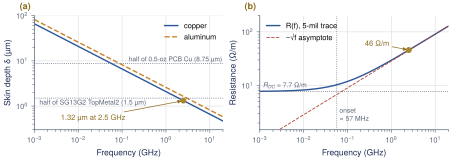
At DC the current fills the whole cross-section of the trace. At high frequency, the changing magnetic field inside the conductor induces eddy currents that cancel the current in the middle, and the current crowds into a surface layer of thickness \[\delta = \sqrt{\frac{\rho}{\pi f \mu_0}}, \tag{3.4}\] the skin depth (\(\rho\) is the resistivity, \(\mu_0 = 4\pi\times10^{-7}\) H/m). For copper (\(\rho = 1.72\times 10^{-8}\,\Omega \,\mathrm{m}\)) at 2.5 GHz, \(\delta = 1.32\,\mu\mathrm{m}\). Once \(\delta\) is below half the conductor thickness, the current flows in a sheet \(\delta\) thick around the effective perimeter \(P\), so \[R(f) \approx \frac{\rho}{P\,\delta} = \frac{\sqrt{\pi f \mu_0 \rho}}{P} \;\propto\; \sqrt f .\] The numerator \(R_s = \rho/\delta\) is the surface resistance in ohms per square. Figure 3.3 shows both effects for a 5-mil (127 µm) wide, half-ounce (17.5 µm) copper trace. On chip, the SG13G2 thick top metals are aluminum, with \(\delta = 1.6\,\mu\mathrm{m}\) at 2.5 GHz, close to half the 3 µm TopMetal2 thickness. That matters for inductors and long clock lines, not for the board channel.
Dielectric loss grows as \(f\)
The alternating field also rotates the dipoles in the board material, and each rotation dissipates a little heat. A lossy dielectric acts like a capacitor with a conductance in parallel, \(G = \omega C \tan\delta\), where the loss tangent \(\tan\delta\) is roughly constant over frequency (0.02 for FR-4, 0.002–0.005 for low-loss laminates). Because \(G\) grows with \(\omega\), dielectric loss grows linearly with frequency. (The loss angle \(\delta\) is unrelated to the skin depth \(\delta\).)
Key equation · Conductor and dielectric attenuation
\[\alpha_R = \frac{R(f)}{2Z_0}, \qquad \alpha_D = \frac{GZ_0}{2} = \frac{\pi f\sqrt{\varepsilon_r}\,\tan\delta}{c} \ [\mathrm{Np/m}], \qquad \mathrm{IL}(f) = 8.686\,(\alpha_R+\alpha_D)\,\ell\ [\mathrm{dB}]. \tag{3.6}\]
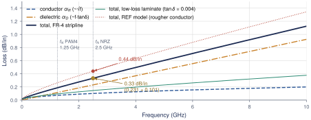
Figure 3.4 plots both terms in dB per inch (1 Np = 8.686 dB). Conductor loss dominates only below about 0.5 GHz. At the 2.5 GHz Nyquist frequency of Open-SERDES, dielectric loss is already more than twice as large, and the gap widens because \(f\) outruns \(\sqrt f\).
Worked Example 3.2 · Loss per inch and reach for a 10 dB budget
Given: the 5-mil, half-ounce, 50 Ω FR-4 stripline of Figure 3.3 (\(\varepsilon_r = 4.0\), \(\tan\delta = 0.02\)) at \(f_\mathrm{N}= 2.5\) GHz.
Dielectric: \(\alpha_D = \pi(2.5\times10^9)(2)(0.02)/(3\times10^8) = 1.047\,\mathrm{Np/m}\): 9.10 dB/m or 0.231 dB/in.
Conductor: \(R_s = \rho/\delta = 13.0\,\mathrm{m\Omega }\) per square. With \(P \approx 2(w+t) = 289\,\mu\mathrm{m}\), \(R \approx 45\,\Omega /\mathrm{m}\), so \(\alpha_R = 45/(2\cdot50) = 0.45\,\mathrm{Np/m}\) or 0.10 dB/in. Copper roughness and return current in the planes add tens of percent in real boards.
Total and reach: \(\alpha \approx 0.33\) dB/in. A 10 dB budget allows \(10/0.33 = 30\) in (76 cm) of bare trace, or 21 in (54 cm) if 3 dB is set aside for two packages and a connector pair. The REF model reaches 10 dB at 0.572 m (22.5 in, the 10 dB entry of LOSS_FAMILY) because its conductor term is twice as large (0.21 dB/in) and it includes the pads.
Why everyone quotes the loss at Nyquist
NRZ puts most of its power below \(f_\mathrm{N}= f_\mathrm{b}/2\) (Section 2.1), and the fastest pattern, 1010…, is a square wave whose fundamental is exactly \(f_\mathrm{N}\). The loss at \(f_\mathrm{N}\) therefore predicts how much the channel closes the eye, and how much equalization you need, far better than the length or the loss at \(f_\mathrm{b}\). For Open-SERDES, budget insertion loss at 2.5 GHz: REF has 17.4 dB. Up to about 10 dB, a small TX FFE or a CTLE is enough; from 10 to 25 dB you need a CTLE and a DFE (Chapter 5).
3.4Reflections and termination
A wave on a line of impedance \(Z_0\) that meets a load \(Z_L\) must satisfy \(V = Z_L I\) at the load and \(V/I = Z_0\) in the wave. One wave cannot do both, so a reflected wave is launched back toward the source, with relative amplitude given by the reflection coefficient.
Key equation · Reflection coefficient and return loss
\[\Gamma_L = \frac{Z_L - Z_0}{Z_L + Z_0}, \qquad \Gamma_S = \frac{R_S - Z_0}{R_S + Z_0}, \qquad V_i = V_S\frac{Z_0}{R_S + Z_0}, \qquad \mathrm{RL} = -20\log_{10}\lvert\Gamma\rvert . \tag{3.7}\]
A matched load gives \(\Gamma = 0\), an open \(+1\) and a short \(-1\). \(V_i\) is the wave launched by a source of open-circuit voltage \(V_S\) and resistance \(R_S\). The return loss RL is \(\lvert\Gamma\rvert\) in positive decibels: larger is better. With both ends mismatched, the wave bounces back and forth. The lattice diagram of Figure 3.5 tracks each bounce, with position across and time down. Each arrival at the load adds \((1+\Gamma_L)\) times the incident wave, and the load voltage converges to the DC divider value only after several round trips of \(2t_d\).
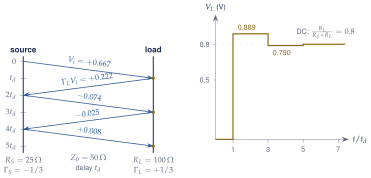
Termination choices
Source termination (\(R_S = Z_0\), open load) absorbs reflections at the driver. Load termination (\(R_L = Z_0\)) absorbs the wave at the receiver but only works if nothing in between reflects. Double termination (\(R_S = R_L = Z_0\)) absorbs every returning echo at either end. It halves the received swing, but echoes are worse than a smaller signal, so serial links use it. Open-SERDES has 50 Ω per side (100 Ω differential) at TX and RX; Section 9.3 builds these resistors in SG13G2. A \(\pm20\%\) resistor error (40–60 Ω) gives \(\lvert\Gamma\rvert \le 0.11\), i.e. RL \(\ge 19\) dB, which is acceptable. The parasitics around the resistor are the bigger problem.
Pad capacitance
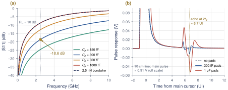
The bond pad, the ESD diodes and the input devices add a shunt capacitance \(C_p\) across the termination. With \(R_T = Z_0\), the load is \(Z_0\parallel 1/(j\omega C_p)\) and Equation (3.7) becomes \[\Gamma(f) = \frac{-j\omega Z_0C_p}{2 + j\omega Z_0C_p}, \qquad \lvert\Gamma\rvert = \frac{\omega Z_0C_p}{\sqrt{4 + (\omega Z_0C_p)^2}} , \tag{3.8}\] plotted in Figure 3.6(a) for several values of \(C_p\).
Worked Example 3.3 · Pad capacitance and return loss
Given: \(R_T = 50\,\Omega\) in parallel with \(C_p = 300\,\mathrm{fF}\) (the REF pad), at 2.5 GHz.
Solution: \(\omega Z_0C_p = 2\pi(2.5\times10^9)(50)(300\times10^{-15}) = 0.236\), so \(\lvert\Gamma\rvert = 0.236/\sqrt{4.056} = 0.117\) and \(\mathrm{RL} = 18.6\,\mathrm{dB}\) (12.8 dB at 5 GHz).
Budget: inverting Equation (3.8), \(\omega Z_0C_p = 2\lvert\Gamma\rvert/\sqrt{1-\lvert\Gamma\rvert^2}\). RL \(\ge 10\) dB at 2.5 GHz allows \(C_p \le 0.85\,\mathrm{pF}\); RL \(\ge 15\) dB allows \(C_p \le 0.46\,\mathrm{pF}\). Pad, ESD and input devices share this budget (Section 9.6).
Worked Example 3.4 · Bondwire inductance
Given: a 2.5 mm bondwire, \(L \approx 2.5\,\mathrm{nH}\) (about 1 nH/mm), in series between two 50 Ω environments, at 2.5 GHz.
Solution: a series impedance \(Z = j\omega L\) between matched lines gives \(S_{11} = (Z/2Z_0)/(1 + Z/2Z_0)\) and \(S_{21} = 1/(1 + Z/2Z_0)\). Here \(\omega L = 39.3\,\Omega\) and \(\omega L/2Z_0= 0.393\). So \(\lvert S_{21}\rvert = 1/\sqrt{1.154} = 0.931\) (\(-0.62\) dB) but \(\lvert S_{11}\rvert = 0.393/1.075 = 0.366\): RL = 8.7 dB, failing a 10 dB target on its own.
Fix: keep bondwires below about 1 mm, use flip-chip bumps, or absorb the inductance into a matched section: 2.5 nH with 1.0 pF of pad capacitance forms an artificial line with \(\sqrt{L/C} = 50\,\Omega\) and a cutoff of \(1/(\pi\sqrt{LC}) = 6.4\) GHz.
Via stubs
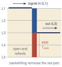
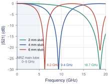
A through-hole via connects traces on different layers. If the signal enters on the top layer and leaves on an inner layer, the rest of the barrel is an unused stub: a short open-ended line hanging off the signal path (Figure 3.7a). Where the stub is a quarter wavelength long, its open end is transformed into a short at the signal path, and almost nothing gets through: \[f_\mathrm{null} \approx \frac{v}{4\,\ell_\mathrm{stub}} . \tag{3.9}\]
Worked Example 3.5 · Via-stub notch
Given: FR-4 (\(v = 1.5\times 10^{8}\,\mathrm{m}/\mathrm{s}\)), stubs of 1.5, 3 and 5 mm.
Solution: Equation (3.9) gives \(f_\mathrm{null} = 25\), 12.5 and 7.5 GHz. To keep the first null above \(3f_\mathrm{N}= 7.5\) GHz, stubs must be shorter than \(v/(4\times7.5\,\mathrm{GHz}) = 5\,\mathrm{mm}\). The barrel’s extra capacitance slows the wave, so in practice keep stubs below about 3 mm, route on layers near the bottom, or backdrill. The Open-SERDES test board should follow this rule for every high-speed via (Section 15.4).
What this means for your design
Every discontinuity sends back a small, filtered copy of the signal. Two discontinuities form a cavity, and the copy that bounces between them reaches the receiver \(2t_d\) late, about 1.7 UI per inch of FR-4 between them. In the pulse response this shows up as ripples and bumps in the tail, often 5–20 UI after the main cursor (Figure 3.6b). A two-tap DFE cannot cancel ISI that far out, so control reflections at the source: accurate termination, small pad capacitance, short bondwires and no long via stubs. A short, low-loss channel does not attenuate its echoes, so it can be harder to equalize than a longer one.
3.5S-parameters
At gigahertz frequencies we cannot measure with opens and shorts, because a short wire is already a transmission line. A vector network analyzer instead drives each port from 50 Ω, terminates the others in 50 Ω, and measures traveling waves: \(a_j\) into port \(j\) and \(b_i\) out of port \(i\). The scattering parameters are \(S_{ij} = b_i/a_j\) with all other inputs matched. For a two-port, \(S_{11}\) is the input reflection (return loss \(-20\log_{10}\lvert S_{11}\rvert\)) and \(S_{21}\) the transmission; the insertion loss is \(\mathrm{IL} = -20\log_{10}\lvert S_{21}\rvert\), a positive number. Because a doubly terminated link has the same 50 Ω reference, \(S_{21}\) is the transfer function \(H_\mathrm{ch}(f) = 2V_\mathrm{out}/V_S\) that we need. To cascade elements, convert each to an ABCD matrix, multiply, and convert back; link.py builds REF this way.
Differential channels and mixed-mode S-parameters
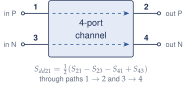
Open-SERDES is differential: the information is \(V_P - V_N\). A differential channel has four single-ended ports, numbered as in Figure 3.8(a): ports 1 and 3 are the P and N inputs, 2 and 4 the P and N outputs. Driving the input differentially (\(a_1 = -a_3\)) and reading the differential output \((b_2 - b_4)/\sqrt2\) gives the mixed-mode parameters, referenced to 100 Ω differential: \[S_{dd21} = \tfrac12\left(S_{21} - S_{23} - S_{41} + S_{43}\right), \qquad S_{dd11} = \tfrac12\left(S_{11} - S_{13} - S_{31} + S_{33}\right). \tag{3.10}\] \(S_{cd21} = \tfrac12(S_{21} - S_{23} + S_{41} - S_{43})\) measures how much differential signal turns into common mode, for example through a P/N length mismatch. For a symmetric, weakly coupled pair, \(S_{dd21}\approx S_{21}\) of one leg, which is why REF can be modeled as a single-ended 50 Ω line.
Crosstalk
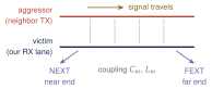
Mutual capacitance \(C_m\) and inductance \(L_m\) couple an aggressor line into a victim (Figure 3.8b). Near-end crosstalk (NEXT) travels back toward the aggressor’s source and is the dangerous kind in a transceiver: a full-swing local TX lane couples into a local RX lane whose own signal has already lost 17 dB. A 0.8 Vppd aggressor at \(-30\) dB NEXT injects about 25 mVpp, comparable with the residual ISI after equalization. Far-end crosstalk (FEXT) travels with the victim’s signal, is attenuated with it, and nearly cancels in a homogeneous stripline. Route TX and RX on different layers or connector rows, and prefer stripline.
Time-domain reflectometry
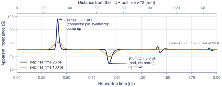
A TDR launches a fast step and records the reflected voltage at the source. A reflection at round-trip time \(t\) comes from distance \(x = vt/2\), and its amplitude gives the local impedance through \(Z = Z_0(1+\rho)/(1-\rho)\), with \(\rho = V_r/V_i\). Figure 3.9 shows the two signature shapes: a series inductance bumps above 50 Ω and a shunt capacitance dips below. For a lumped element, the size of the feature depends on the rise time: with a 25 ps step a 1 nH pin reads 97 Ω, with a 100 ps step only 61 Ω. A TDR result always comes with its rise time, which sets its resolution.
3.6From frequency to time
The tools of Chapter 4 need the pulse response \(p(t)\) of Section 2.4. We get it from \(S_{21}(f)\) in two steps.
Causality
A physical channel cannot respond before it is driven. In the frequency domain this means the magnitude and phase of \(H_\mathrm{ch}(f)\) are linked: a given loss curve comes with a specific phase (dispersion). A model built from \(\lvert S_{21}\rvert\) alone with a pure delay gives a symmetric impulse response that starts long before the wave could arrive (Figure 3.10). A dielectric model with \(\varepsilon_r\) and \(\tan\delta\) held exactly constant has the same flaw in a milder form. REF uses a causal dielectric whose capacitance varies as \((j\omega/\omega_0)^{-2\tan\delta/\pi}\), the simplest of the causal FR-4 models [17]. A non-causal model produces fake pre-cursors, which then mislead the design of the TX FFE pre-tap.
Impulse and pulse response
The impulse response is the inverse Fourier transform of the conjugate-symmetric spectrum, \(h(t) = \mathcal F^{-1}\{H_\mathrm{ch}(f)\}\) with \(H_\mathrm{ch}(-f) = H_\mathrm{ch}^*(f)\). The pulse response is \(h(t)\) convolved with a 1-UI rectangle.
Key equation · From \(S_{21}\) to the pulse response
\[p(t) = \int_{t-T_\mathrm{b}}^{t} h(\tau)\,d\tau \;\;\Longleftrightarrow\;\; P(f) = H_\mathrm{ch}(f)\,T_\mathrm{b}\,\mathrm{sinc}(fT_\mathrm{b})\,e^{-j\pi fT_\mathrm{b}} \tag{3.11}\]
On a grid of \(N\) points spaced \(\Delta f\) up to \(f_\mathrm{max}\), the IFFT gives a time step \(\Delta t = 1/(2f_\mathrm{max})\) and a window \(T_w = 1/\Delta f\). common.py uses 0–160 GHz in 10 MHz steps: \(\Delta t = 3.125\,\mathrm{ps}\) (64 samples per UI) and \(T_w = 100\,\mathrm{ns}\), far longer than the REF delay plus tail. Figure 3.11 compares the two responses: the 1-UI rectangle averages \(h\) over 200 ps, so \(p(t)\) is smoother and lower, and its tail coincides with that of \(h(t)\cdot T_\mathrm{b}\).
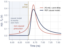
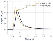
Figure 3.12 shows how the pulse response changes with loss, using the LOSS_FAMILY lines of link.py. From 5 to 25 dB of Nyquist loss, the main cursor falls from 0.77 to 0.22 V while the first post-cursor stays near 0.16–0.18 V, so \(p_1/p_0\) grows from 0.12 to 0.71. That ratio, more than the loss itself, is what the equalizer must fight.
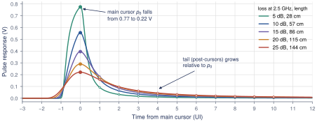
LOSS_FAMILY channels, aligned at their peaks; open dots mark the post-cursors \(p_1\ldots p_{10}\). At 15 dB (close to REF) the first post-cursor is already 46% of the main cursor.IFFT mistakes that change your cursors
Forgetting conjugate symmetry gives a complex \(h(t)\). A coarse \(\Delta f\) makes the window shorter than the delay plus tail, so the tail wraps around and looks like pre-cursor ISI. Data cut abruptly at its last frequency rings (Gibbs), and data without a DC point must be extrapolated. And the cursors are samples of \(p(t)\), not of \(h(t)\).
3.7The Open-SERDES reference channel
Every model, figure and lab in this book uses one synthetic channel, REF: a 50 Ω source, a 300 fF pad, 1 m of lossy FR-4 stripline, another 300 fF pad and a 50 Ω load. It is built from serdespy’s ABCD functions [3] by channel(1.0) in tutorial/figsrc/link.py and tutorial/code/common.py. Table 3.1 lists the parameters, and Figure 3.13 shows the insertion loss: −17.4 dB at 2.5 GHz. The pads cost only 0.1 dB of that; their real damage is the reflections they add.
Table 3.1. REF model parameters and the matching channel() arguments.
| Quantity | Value | Arg. |
|---|---|---|
| Length | 1.0 m | length |
| \(Z_0\) per side | 50 \(\Omega\) | z0 |
| \(\varepsilon_r\) | 4.0 (6.67 ns/m) | er |
| \(\tan\delta\) | 0.02 at 1 GHz, causal | tand |
| \(R_\mathrm{DC}\) | 7 \(\Omega\)/m | rdc |
| Skin \(R\) | 60 \(\Omega\)/m at 1 GHz, \(\propto\!\sqrt f\) | kr |
| Pads | 300 fF each end | c_pad |
| Source, load | 50 \(\Omega\) each | |
| Grid | 0–160 GHz, 10 MHz | F |
| Loss | 0.59 / 10.4 / 17.4 / 30.1 dB | |
| at 0 / 1.25 / 2.5 / 5 GHz |
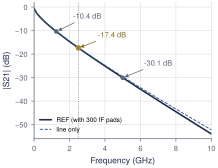
Figure 3.14 shows the REF pulse response sampled every UI from its peak, and Table 3.2 lists the cursors. These thirteen numbers are the most-used data in this book.
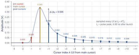
| \(k\) | \(-2\) | \(-1\) | \(\mathbf{0}\) | 1 | 2 | 3 | 4 | 5 | 6 | 7 | 8 | 9 | 10 |
|---|---|---|---|---|---|---|---|---|---|---|---|---|---|
| \(p_k\) | 0.000 | 0.0486 | 0.3396 | 0.1817 | 0.0909 | 0.0537 | 0.0356 | 0.0255 | 0.0192 | 0.0150 | 0.0121 | 0.0100 | 0.0084 |
Why this channel is hard
Three numbers tell the story. First, \(p_0 = 0.34\): only a third of the transmitted pulse arrives in its own UI. Second, \(p_1/p_0 = 0.535\): the previous bit contributes more than half as much as the current one. Third, the ISI magnitudes \(\sum_{k\ne0}\lvert p_k\rvert\) of these cursors add up to 0.501 V, more than \(p_0\). A worst-case pattern can push a “1” below zero, and the peak-distortion eye of Section 4.2 is \(1\,\mathrm{V}\times(0.340 - 0.501) = -0.161\) V: closed. A PRBS7 simulation agrees (Section 16.3). REF cannot be received without equalization, and the Open-SERDES link must still reach BER \(\le 10^{-12}\) over it, with margin up to the 20–25 dB end of LOSS_FAMILY (Section 8.5, Table 14.2).
Replacing REF with real S-parameters
REF is a teaching model. Once the Open-SERDES test board is measured, or its traces are simulated with openEMS or Palace, you will swap in a 4-port Touchstone file. scikit-rf [18] reads it, converts it to mixed mode and extrapolates it to DC; the rest of the flow is unchanged:
import skrf as rf
from common import *                       # grid F, impulse(), pulse(), SPS
ch = rf.Network("board.s4p")               # measured or EM-simulated 4-port
ch.renumber([1, 2], [2, 1])                # book map (1,3 in; 2,4 out) -> skrf (0,1 in)
ch.se2gmm(p=2)                             # mixed mode: ports d-in, d-out, c-in, c-out
ch = ch.extrapolate_to_dc(kind="linear")   # add 0 Hz, uniform frequency step
sdd21 = ch.s[:, 1, 0]
H = np.interp(F, ch.f, sdd21.real, right=0) + 1j * np.interp(F, ch.f, sdd21.imag, right=0)
h, t = impulse(H); p = pulse(h)            # then cursors(), pda_eye(), ... as for REF
Check the port map first (Figure 3.8), and taper the data toward its highest frequency instead of cutting it to zero. serdespy’s four_port_to_diff does the same job but assumes through paths \(1\to2\) and \(3\to4\) and ignores its port_def argument.
Lab 1: the channel
Run lab1_channel.py (Section 16.2). It plots \(\lvert S_{21}\rvert\) of REF, converts it to \(h(t)\) and \(p(t)\), and prints the cursors of Table 3.2. Then set c_pad to 1 pF and length to 0.3 m and watch the reflections of Figure 3.6(b) appear in the tail.
3.8Exercises
Is it a line? A package trace is 8 mm long on a substrate with \(\varepsilon_r = 3.5\), driven with \(t_r = 40\,\mathrm{ps}\). Compute its delay. Must it be modeled as a transmission line?
Better laminate. Repeat Worked Example 3.2 for a low-loss laminate (\(\varepsilon_r = 3.7\), \(\tan\delta = 0.004\)) with the same copper. How long can the trace be for 17.4 dB at 2.5 GHz? Which loss term now dominates?
ESD budget. The RX must have RL \(\ge 15\) dB at 2.5 GHz. The pad is 120 fF and the input devices add 60 fF. How much capacitance is left for ESD protection?
Via stub. A 3.2 mm thick board routes a signal from L1 to an inner layer 0.8 mm deep, and the via’s capacitance gives \(\varepsilon_{r,\mathrm{eff}} = 6\). Where is the stub null? Is it acceptable for Open-SERDES? What if the signal exits on the bottom layer instead?
Cursor ratio. With
channel()fromlink.py, find the length at which \(p_1/p_0 = 0.5\) and its Nyquist loss. Repeat withtand=0.01and explain why the answer moves.
Key takeaways
Off-chip, every trace longer than about 1 mm is a transmission line at 5 Gb/s. FR-4 delay is 6.67 ps/mm (169 ps/in); REF takes 6.67 ns, or 33 UI.
Conductor loss grows as \(\sqrt f\) (skin depth 1.32 m at 2.5 GHz); dielectric loss grows as \(f\tan\delta\) and dominates FR-4 above 0.5 GHz. A smooth FR-4 stripline loses about 0.33 dB/in at 2.5 GHz.
Quote and budget insertion loss at Nyquist, 2.5 GHz. REF loses 17.4 dB there.
Discontinuities reflect: 300 fF of pad gives RL = 18.6 dB, a 2.5 nH bondwire only 8.7 dB, and a via stub notches \(S_{21}\) at \(v/(4\ell)\). Echoes return as late bumps in the pulse response.
Use mixed-mode \(S_{dd21}\) for differential channels and check the port map. On a TDR, inductance bumps up and capacitance dips down.
A causal model and a correct IFFT turn \(S_{21}\) into \(h(t)\) and \(p(t)\). REF has \(p_{-1} = 0.049\), \(p_0 = 0.340\) and \(p_1 = 0.182\) (\(p_1/p_0 = 0.535\)), and its unequalized peak-distortion eye is closed (\(-0.161\) V).
Generated from book/tutorial/chapters/03_channel.tex. Figure, table and equation numbers match the PDF edition.