Chapter 7Continuous-Time Linear Equalizer
A CTLE is a high-pass filter built into the first receiver stage. It lifts the frequencies the channel attenuated by giving up gain at low frequencies.
In this chapter you will learn
Compare passive RC, RLC and degenerated-pair CTLEs and know why the degenerated pair is the workhorse.
Derive the degenerated-pair transfer function, with its zero, two poles, DC gain and peaking.
Turn a peaking target into \(R_S\), \(C_S\), \(R_D\) and \(C_\mathrm{L}\), and respect the gain–bandwidth limit.
Choose the peaking for the REF channel, and recognize over-peaking.
Design an SG13G2 HBT CTLE, explain why its realized boost falls short of the ideal, and make it programmable from 0 to 12 dB.
7.1From RC to RLC: three passive ideas
The channel is a low-pass filter, so its inverse must be a high-pass filter. Figure 7.1 shows three passive ways to build one.
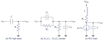
RC high-pass
\(H(s)=sRC/(1+sRC)\) has zero gain at DC. A long run of identical bits decays toward 0 V, so the baseline wanders with the data. On its own it is unusable.
Over-compensated divider
With a series \(R_1\Vert C_1\) and a shunt \(R_2\Vert C_2\), \[H(s)=\frac{R_2}{R_1+R_2}\cdot\frac{1+sR_1C_1}{1+s\,(R_1\Vert R_2)(C_1+C_2)},\qquad \frac{\omega_p}{\omega_z}=\frac{R_1+R_2}{R_2}\cdot\frac{C_1}{C_1+C_2}. \tag{7.1}\] The DC gain is \(R_2/(R_1+R_2)\) and the high-frequency gain is \(C_1/(C_1+C_2)\). With \(R_1C_1=R_2C_2\) it is a flat compensated probe; a larger \(R_1C_1\) makes it an equalizer. It is very linear, but its gain is below 1 everywhere, which degrades the SNR at the next stage.
RLC load
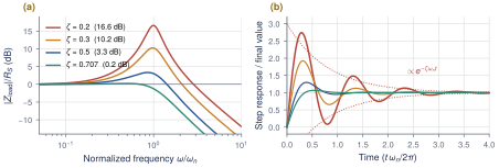
Put an inductor in series with the load resistor \(R_S\) of a differential pair and let \(C\) be the node capacitance. With \(\omega_n=1/\sqrt{LC}\) and \(\zeta=\tfrac{R_S}{2}\sqrt{C/L}\), the load impedance is \[Z(s)=R_S\,\frac{\omega_n}{2\zeta}\cdot\frac{s+2\zeta\omega_n}{s^2+2\zeta\omega_n s+\omega_n^2},\qquad \frac{\lvert Z(j\omega_n)\rvert}{R_S}=\frac{\sqrt{1+4\zeta^2}}{4\zeta^2}. \tag{7.2}\] With \(\zeta=0.2\) the boost is 6.7, or 16.6 dB (Figure 7.2). That is a serious drawback: the complex poles sit close to the \(j\omega\) axis, so the step response rings as \(e^{-\zeta\omega_nt}\cos(\sqrt{1-\zeta^2}\,\omega_nt)\), and the ringing is ISI of its own. Mild inductive peaking with \(\zeta\approx0.5\)–0.7 is still useful. It extends bandwidth without much ringing, and we return to it in Section 7.4.
7.2The source-degenerated differential pair
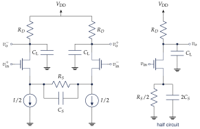
The workhorse CTLE is a differential pair with a parallel \(R_S\Vert C_S\) between its sources or emitters (Figure 7.3). At low frequency \(R_S\) degenerates the pair and lowers its gain. At high frequency \(C_S\) shorts \(R_S\), and the full gain \(g_\mathrm{m}R_D\) returns. The zero and first pole are set by \(R_S\) and \(C_S\), so \(R_S\) can be a triode MOSFET and \(C_S\) a varactor, giving a tunable CTLE [22].
Transfer function of the degenerated pair
In the half circuit the source sees \(Z_S=\tfrac{R_S}{2}\big\Vert\tfrac{1}{2sC_S}=\dfrac{R_S/2}{1+sR_SC_S}\). Series feedback divides the transconductance by \(1+g_\mathrm{m}Z_S\): \[G_m(s)=\frac{g_\mathrm{m}}{1+g_\mathrm{m}Z_S}=\frac{g_\mathrm{m}\,(1+sR_SC_S)}{1+g_\mathrm{m}R_S/2+sR_SC_S} =\frac{g_\mathrm{m}}{1+g_\mathrm{m}R_S/2}\cdot\frac{1+sR_SC_S}{1+\dfrac{sR_SC_S}{1+g_\mathrm{m}R_S/2}} .\] The drain load is \(Z_D=R_D/(1+sR_DC_\mathrm{L})\), and \(H=G_mZ_D\) (the sign inversion is absorbed by the output polarity).
Key equation · Degenerated-pair CTLE
\[\begin{gathered} H_\mathrm{CTLE}(s)=\frac{g_\mathrm{m}R_D}{1+g_\mathrm{m}R_S/2}\cdot\frac{1+s/\omega_z}{(1+s/\omega_{p1})(1+s/\omega_{p2})},\\[2pt] \omega_z=\frac{1}{R_SC_S},\qquad \omega_{p1}=\frac{1+g_\mathrm{m}R_S/2}{R_SC_S},\qquad \omega_{p2}=\frac{1}{R_DC_\mathrm{L}} \end{gathered} \tag{7.3}\] DC gain \(=g_\mathrm{m}R_D/(1+g_\mathrm{m}R_S/2)\). Gain between \(\omega_{p1}\) and \(\omega_{p2}\) \(\approx g_\mathrm{m}R_D\). Ideal peaking \(=\omega_{p1}/\omega_z=1+g_\mathrm{m}R_S/2\).
\(R_S\) sets the peaking and the DC gain, and barely moves \(\omega_{p1}\approx g_\mathrm{m}/(2C_S)\) when \(g_\mathrm{m}R_S/2\gg1\). \(C_S\) moves \(\omega_z\) and \(\omega_{p1}\) together at constant peaking (Figure 7.4a). In this book the “peaking” of a setting means the ideal ratio \(\omega_{p1}/\omega_z\), as in ctle() of link.py, which fixes \(f_{p1}=f_\mathrm{N}\), \(f_{p2}=10\,\mathrm{GHz}\) and 0 dB high-frequency gain. The boost realized at \(f_\mathrm{N}\) is smaller: the 12 dB setting gives 9.0 dB, because the first pole already costs 3 dB there (Figure 7.4b).
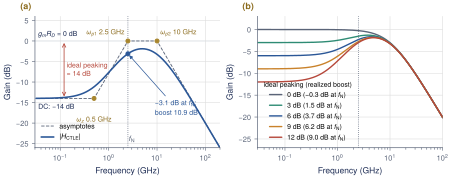
ctle() family from 0 to 12 dB, as used in the REF studies. The legend gives the boost realized at \(f_\mathrm{N}\).Worked Example 7.1 · From a peaking target to component values
Lab 4 finds 14 dB best for REF without a DFE (Section 7.3). Target \(a=10^{14/20}=5.01\), \(f_{p1}=f_\mathrm{N}\), \(f_{p2}=10\,\mathrm{GHz}\) and 0 dB high-frequency gain, with \(g_\mathrm{m}=20\,\mathrm{mS}\) per side. Peaking: \(R_S=2(a-1)/g_\mathrm{m}=401\,\Omega\). Zero: \(f_z=f_{p1}/a=0.499\,\mathrm{GHz}\), so \(C_S=1/(2\pi f_zR_S)=0.795\,\mathrm{pF}\). Gain: \(g_\mathrm{m}R_D=1\) gives \(R_D=50\,\Omega\), and \(C_\mathrm{L}=1/(2\pi f_{p2}R_D)=318\,\mathrm{fF}\). The DC gain is \(g_\mathrm{m}R_D/a=0.20\) (−14 dB). This circuit only loses gain at low frequency; a real front end adds gain with more \(g_\mathrm{m}R_D\) or a following stage.
Gain–bandwidth
Multiplying the mid-band gain by the second pole gives \[(g_\mathrm{m}R_D)\cdot\omega_{p2}=\frac{g_\mathrm{m}}{C_\mathrm{L}}. \tag{7.4}\] This is the gain–bandwidth product of a plain differential pair; degeneration does not change it. A high \(\omega_{p2}\) together with a large peak gain needs more \(g_\mathrm{m}\) (current) or a smaller \(C_\mathrm{L}\) (smaller next stage, inductive peaking).
7.3The CTLE on the REF channel
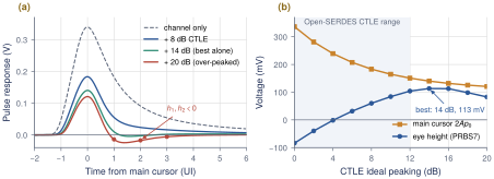
Lab 4 cascades REF with ctle(pk) and sweeps the peaking (Figure 7.5). Without a CTLE the PRBS7 eye is −84 mV. It opens at about 4 dB, reaches 104 mV at 12 dB and peaks at 113.3 mV (0.94 UI) at 14 dB. Beyond 16 dB it closes again. Meanwhile the main cursor \(2Ap_{0}\) falls steadily, from 337 mV to 140 mV at 14 dB. This is the CTLE “boosting” by suppressing the low frequencies.
What this means for your design
Over-peaking returns the ISI with the opposite sign. Above 16 dB, \(p_{1}\) and \(p_{2}\) turn negative and the eye closes again.
Every dB of peaking costs main cursor. From 0 to 14 dB the main cursor drops by 7.6 dB. Noise that enters after the CTLE, such as sampler and DFE-summer noise, does not drop with it, and the CTLE’s high-frequency gain lifts noise and crosstalk relative to the signal.
Pre-cursors shrink but do not vanish. In our model \(p_{-1}\) falls from 0.049 to 0.006 at 14 dB. A larger pre-cursor, for example from a reflection, is a job for the TX pre-tap.
With a DFE behind it, the CTLE should be tuned for the best eye after the DFE. Let the DFE take \(p_{1}\) instead of peaking it away (Section 8.5).
Lab 4: CTLE
lab4_ctle.py sweeps the peaking from 0 to 20 dB, prints the eye and the cursors, and converts the best setting into \(R_S\), \(C_S\), \(R_D\) and \(C_\mathrm{L}\) (Section 16.5).
7.4An HBT CTLE in SG13G2
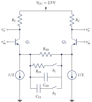
Open-SERDES builds its CTLE from SG13G2 SiGe HBTs. A bipolar transistor gives \(g_\mathrm{m}=I_C/V_T=38.7\,\mathrm{mS}\) per mA, several times more than a MOSFET at the same current, and its \(f_T\approx300\,\mathrm{GHz}\) keeps device capacitance small. The circuit is Figure 7.3 with npn devices, emitter degeneration \(R_E\Vert C_E\) and collector loads \(R_C\). Each \(V_{CE}\) must stay below the \(\mathrm{BV}_{CEO}\) of about 1.6–1.7 V on the 2.5 V analog supply.
Worked Example 7.2 · An SG13G2 HBT CTLE with 10 dB of ideal peaking
Bias with \(I_\mathrm{tail}=2\,\mathrm{mA}\) (1 mA per side): \(g_\mathrm{m}=1\,\mathrm{mA}/25.85\,\mathrm{mV}=38.7\,\mathrm{mS}\).
10 dB ideal peaking: \(1+g_\mathrm{m}R_E/2=3.16\), so \(R_E=2(2.16)/g_\mathrm{m}=112\,\Omega\).
Put \(f_{p1}\) at \(f_\mathrm{N}\): \(f_z=2.5/3.16=0.79\,\mathrm{GHz}\), so \(C_E=1/(2\pi f_zR_E)=1.8\,\mathrm{pF}\).
\(R_C=200\,\Omega\) and \(C_\mathrm{L}=100\,\mathrm{fF}\) give \(f_{p2}=7.96\,\mathrm{GHz}\).
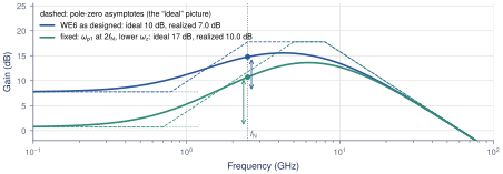
DC gain \(=g_\mathrm{m}R_C/3.16=2.45\) (7.8 dB). \(\lvert H(j2\pi f_\mathrm{N})\rvert=14.8\,\mathrm{dB}\).
The realized boost at \(f_\mathrm{N}\) is \(14.8-7.8=7.0\,\mathrm{dB}\), not 10 dB. Each factor of Equation (7.3) evaluated at \(f_\mathrm{N}\) shows why: the zero contributes \(20\log_{10}\lvert1+j\,2.5/0.79\rvert=+10.4\) dB, the first pole \(-3.0\) dB because it sits at \(f_\mathrm{N}\), and the second pole \(-0.4\) dB. The response peaks at 4.3 GHz, well above \(f_\mathrm{N}\).
Fix. The boost at \(f_\mathrm{N}\) is set by \(f_\mathrm{N}/f_z\), minus whatever the poles take away. Move \(f_{p1}\) up to \(2f_\mathrm{N}\) and lower \(f_z\) to 0.70 GHz. That needs \(1+g_\mathrm{m}R_E/2=7.1\) (17 dB ideal), so \(R_E=317\,\Omega\) and \(C_E=0.72\,\mathrm{pF}\). The realized boost is then 10.0 dB. The price is DC gain, which falls to 0.7 dB (Figure 7.6). A second option is inductive (shunt) peaking in the collector loads. It pushes \(\omega_{p2}\) out and adds a little gain near \(f_\mathrm{N}\) (Section 7.1).
Programmability
The Open-SERDES CTLE must cover 0–12 dB of peaking for channels shorter and longer than REF. Figure 7.7 shows the usual way to do it: binary-weighted banks of \(R_E\) and \(C_E\) segments, switched in parallel by MOS switches under a digital code. Closing more \(R_E\) segments lowers \(R_{E,\mathrm{eff}}\), which reduces the peaking and raises the DC gain. A fully closed bank (0 dB) makes it a flat amplifier. \(C_E\) segments are switched together with \(R_E\), so \(\omega_{p1}\) stays near \(2f_\mathrm{N}\). Keep the switches small. Their on-resistance adds to \(R_E\) and their junction capacitance adds to \(C_E\), and both shift the corners. Include them in the ngspice netlist.
Noise
The degeneration resistor adds \(\sqrt{4kTR_E}=1.4\,\mathrm{nV}/\sqrt{\mathrm{Hz}}\) for \(R_E=112\,\Omega\), against \(\sqrt{2\cdot2kT/g_\mathrm{m}}=0.65\,\mathrm{nV}/\sqrt{\mathrm{Hz}}\) of collector shot noise from the pair. Over 5 GHz that is about 0.1 mV rms, far below the 10 mV slicer noise assumed in Lab 5. Offset, crosstalk and linearity limit a 5 Gb/s CTLE before thermal noise does.
Linearity and overload
With a split tail, the pair fully switches when the differential input exceeds about \(I_\mathrm{tail}R_E/2\) plus a few \(V_T\). For Worked Example 7.2 that is \(112+\sim100\approx0.2\,\mathrm{V}\). Long runs on REF arrive at nearly the full DC level, \(\pm0.93\times0.5\,\mathrm{V}=\pm0.47\,\mathrm{V}\) differential. The CTLE would compress them, and a compressed CTLE breaks the linear superposition that the DFE taps rely on. Three remedies stack: TX de-emphasis lowers the long-run level (\(\pm0.23\,\mathrm{V}\) at \(-6\) dB); the fixed design’s \(I_\mathrm{tail}R_E/2=317\,\mathrm{mV}\) widens the linear range; and an input attenuator or gain control handles short channels (Section 10.1). At high frequency \(C_E\) shorts \(R_E\) and the range shrinks toward that of a bare pair, about \(\pm2V_T\). That is tolerable, because the channel has already attenuated the high-frequency content by 17 dB.
Open-SERDES CTLE targets (derived here)
Ideal peaking 0–12 dB in 1–2 dB steps (\(\approx9\) dB realized at \(f_\mathrm{N}\)); \(f_{p1}\approx1\)–\(2\,f_\mathrm{N}\); \(f_{p2}\ge7.5\,\mathrm{GHz}\); DC gain \(\ge0\) dB at 12 dB; LF linear range \(\ge\pm0.25\,\mathrm{V}\) differential. Verify the realized boost in ngspice.
Key takeaways
An RC high-pass has no DC gain and a passive divider has no gain at all. RLC peaking gives boost but rings when \(\zeta\) is small (16.6 dB at \(\zeta=0.2\)).
The degenerated pair gives \(\omega_z=1/R_SC_S\), \(\omega_{p1}=(1+g_\mathrm{m}R_S/2)/R_SC_S\) and \(\omega_{p2}=1/R_DC_\mathrm{L}\), with ideal peaking \(1+g_\mathrm{m}R_S/2\).
The CTLE boosts by suppressing the low frequencies. Its gain–bandwidth is still \(g_\mathrm{m}/C_\mathrm{L}\).
On REF, the eye is best at 14 dB without a DFE (113.3 mV). Over-peaking turns the post-cursors negative and costs main cursor.
Realized boost at \(f_\mathrm{N}\) is well below the ideal when \(f_{p1}=f_\mathrm{N}\): 7.0 dB instead of 10 dB in Worked Example 7.2. Move \(f_{p1}\) up and \(f_z\) down to recover it.
Make the HBT CTLE programmable with switched \(R_E\)/\(C_E\) banks, and check its linear range against the long-run input level.
Generated from book/tutorial/chapters/07_ctle.tex. Figure, table and equation numbers match the PDF edition.