Chapter 12Clock Generation:
The Phase-Locked Loop
A crystal gives a clean 50 MHz; the link needs a clean 2.5 GHz in four phases. The charge-pump PLL with an LC VCO bridges the two.
In this chapter you will learn
Explain how a phase-frequency detector and charge pump turn a timing error into charge, and why the reset delay removes the dead zone.
Derive the type-II loop’s \(\omega_n\) and \(\zeta\), and design the Open-SERDES loop filter for a given bandwidth and phase margin.
Use noise transfer functions to choose the loop bandwidth that minimizes output jitter.
Size an LC tank, state the oscillation condition, and use Leeson’s model to sanity-check a phase-noise number.
Generate and distribute quadrature (I/Q) clocks, and budget their phase and duty-cycle errors.
12.1The charge-pump PLL
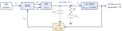
A free-running VCO drifts: its TIE random-walks (Figure 11.1b) and its frequency wanders with temperature and supply. A phase-locked loop (PLL) fixes both by comparing the divided VCO output with a crystal reference and steering the VCO until the two are aligned. Gardner’s analysis of the charge-pump PLL [35] underlies this chapter; Razavi [36], Gardner’s book [37] and ECEN 720 [34] treat it in more depth. Locked, the output frequency is exactly \(N f_\mathrm{ref}\). Open-SERDES uses an integer-N charge-pump PLL (Figure 12.1) with \(f_\mathrm{ref} = 50\) MHz and \(N = 50\), reusing the team’s LC-VCO PLL design [9] retuned from 2.4 to 2.5 GHz.
Phase-frequency detector and charge pump
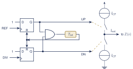
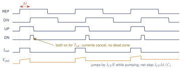
The PFD is two flip-flops with their D inputs tied high (Figure 12.2). A rising reference edge sets UP, a rising divider edge sets DN, and when both are high an AND gate resets them after a short delay \(T_\mathrm{rst}\). The width of UP minus the width of DN equals the timing difference \(\Delta t\) between the edges. If the frequencies differ, one output dominates for many cycles, so the PFD also pulls the frequency in: it is a phase and frequency detector. The charge pump switches a current \(I_\mathrm{CP}\) into the loop filter during UP and out during DN. The average current is \(I_\mathrm{CP}\,\Delta t/T_\mathrm{ref} = I_\mathrm{CP}\,\Delta\phi/2\pi\), so the PFD-plus-CP gain is \(I_\mathrm{CP}/2\pi\) amperes per radian of reference phase.
Dead zone and mismatch
Without the reset delay, a tiny \(\Delta t\) would give UP and DN pulses too short to switch the charge pump on, so near lock the loop would get no correction: a dead zone in which the VCO drifts. With \(T_\mathrm{rst}\) of 100–200 ps both pulses always last at least \(T_\mathrm{rst}\), and the net charge stays proportional to \(\Delta t\) down to zero. The price is mismatch: if the currents differ by \(\Delta I\), the loop locks at a static offset \(\Delta t = (\Delta I/I_\mathrm{CP})\,T_\mathrm{rst}\) (7.5 ps for 5% and 150 ps), and the current pulses every 20 ns create a reference spur, a periodic jitter that \(C_2\) and the loop must filter.
12.2Loop dynamics
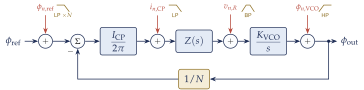
Near lock every block is linear in phase, which gives the model of Figure 12.3. The PFD and CP give \(I_\mathrm{CP}/2\pi\) (A/rad); the loop filter impedance \(Z(s)\) turns current into \(V_\mathrm{ctrl}\); the VCO integrates frequency into phase, \(K_\mathrm{VCO}/s\) (rad/s/V divided by \(s\)); and the divider scales phase by \(1/N\). The same figure marks where each noise source enters.
Type-II second-order loop
Ignore \(C_2\) for now, so \(Z(s) = R + 1/(sC_1)\). The open-loop gain is \[LG(s) = \frac{I_\mathrm{CP}}{2\pi}\,Z(s)\,\frac{K_\mathrm{VCO}}{s}\,\frac1N = \frac{I_\mathrm{CP}K_\mathrm{VCO}}{2\pi N C_1}\cdot\frac{1 + sRC_1}{s^2} .\] It has two integrators (the VCO and \(C_1\)), so it is a type-II loop: it settles to zero phase error even after a frequency step. The closed-loop transfer \(\phi_\mathrm{out}/\phi_\mathrm{ref} = N\,LG/(1+LG)\) becomes, after multiplying through by \(s^2\),
Key equation · CP-PLL natural frequency and damping
\[\frac{\phi_\mathrm{out}}{\phi_\mathrm{ref}} = N\,\frac{2\zeta\omega_n s + \omega_n^2}{s^2 + 2\zeta\omega_n s + \omega_n^2}, \qquad \omega_n = \sqrt{\frac{I_\mathrm{CP}K_\mathrm{VCO}}{2\pi N C_1}}, \qquad \zeta = \frac{R}{2}\sqrt{\frac{I_\mathrm{CP}K_\mathrm{VCO}C_1}{2\pi N}} . \tag{12.1}\]
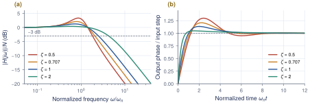
Matching coefficients gives \(\omega_n^2 = I_\mathrm{CP}K_\mathrm{VCO}/(2\pi N C_1)\) and \(2\zeta\omega_n = I_\mathrm{CP}K_\mathrm{VCO}R/(2\pi N)\). Raising \(R\) raises the damping without changing \(\omega_n\); raising \(C_1\) lowers \(\omega_n\) and raises \(\zeta\). The zero in the numerator causes some jitter peaking at every damping (Figure 12.4, Table 12.1): the loop amplifies reference jitter near \(\omega_n\). The \(-3\) dB bandwidth is \(\omega_{-3\mathrm{dB}} = \omega_n\big[1 + 2\zeta^2 + \sqrt{(1+2\zeta^2)^2 + 1}\,\big]^{1/2}\), which tends to \(2\zeta\omega_n\) for large \(\zeta\).
| \(\zeta\) | 0.5 | 0.707 | 1 | 2 | 4 | 4.5 |
|---|---|---|---|---|---|---|
| \(\omega_{-3\mathrm{dB}}/\omega_n\) | 1.82 | 2.06 | 2.48 | 4.25 | 8.13 | 9.11 |
| Peaking (dB) | 3.3 | 2.1 | 1.25 | 0.40 | 0.12 | 0.09 |
The third pole and phase margin
The capacitor \(C_2\) in parallel smooths the voltage step \(I_\mathrm{CP}R\) seen in Figure 12.2, which would otherwise modulate the VCO every reference cycle. It adds a pole at \(\omega_{p3} = 1/(R C_s)\) with \(C_s = C_1C_2/(C_1+C_2)\), and the loop becomes third order. The usual design places the unity-gain frequency \(\omega_u\) at the geometric mean of the zero \(\omega_z = 1/(RC_1)\) and \(\omega_{p3}\), where the phase margin \(\Phi_m\) is largest. With \(K_C = C_1/C_2\): \[\begin{gathered} K_C = 2\tan^2\Phi_m + 2\tan\Phi_m\sqrt{\tan^2\Phi_m + 1}, \qquad \omega_z = \frac{\omega_u}{\sqrt{1+K_C}}, \qquad \omega_{p3} = \omega_u\sqrt{1+K_C}, \\ C_2 = \frac{I_\mathrm{CP}K_\mathrm{VCO}}{2\pi N\omega_u^2}\sqrt{\frac{\omega_u^2+\omega_z^2}{\omega_u^2+\omega_{p3}^2}}, \qquad C_1 = K_C C_2, \qquad R = \frac{1}{\omega_z C_1} . \end{gathered} \tag{12.2}\] For \(\Phi_m = 60^\circ\), \(K_C = 12.9\). Keep \(f_u \le f_\mathrm{ref}/10\), or the sampled nature of the PFD makes the continuous-time model wrong.
Worked Example 12.1 · Loop filter for the Open-SERDES PLL
Given: \(f_\mathrm{ref} = 50\) MHz, \(N = 50\), \(K_\mathrm{VCO}= 2\pi\times150\) MHz/V, \(I_\mathrm{CP}= 200\) A, \(f_u = 1\) MHz, \(\Phi_m = 60^\circ\).
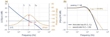
Pole and zero: \(K_C = 12.93\), so \(f_z = 1\,\mathrm{MHz}/\sqrt{13.93} = 268\) kHz and \(f_{p3} = 3.73\) MHz. Components from Equation (12.2): \(C_2 = \mathbf{4.07}\) pF, \(C_1 = K_C C_2 = \mathbf{52.6}\) pF, \(R = 1/(\omega_z C_1) = \mathbf{11.3}\) k\(\Omega\). Check with Equation (12.1): \(f_n = 537\) kHz and \(\zeta = 1.00\). The full third-order loop, simulated in Python (Figure 12.5), crosses unity gain at 1.00 MHz with 60.0\(^\circ\) margin and has \(f_{-3\mathrm{dB}} = 1.56\) MHz with 1.7 dB peaking. Practical: \(f_\mathrm{ref}/f_u = 50\), comfortably above 10. \(C_1\) is 0.035 mm\(^2\) of MIM at about 1.5 fF/m\(^2\) (check the PDK value), the largest item in the PLL layout. \(R\) adds \(\sqrt{4kTR} = 13.7\) nV/\(\sqrt{\mathrm{Hz}}\) of band-pass noise.
12.3PLL noise and the optimum bandwidth
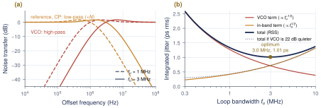
From Figure 12.3, each noise source sees its own transfer function: \[\mathrm{NTF}_\mathrm{ref} = N\frac{LG}{1+LG}, \quad \mathrm{NTF}_\mathrm{CP} = \frac{2\pi}{I_\mathrm{CP}}\,N\frac{LG}{1+LG}, \quad \mathrm{NTF}_\mathrm{VCO} = \frac{1}{1+LG}, \quad \mathrm{NTF}_R = \frac{K_\mathrm{VCO}/s}{1+LG} .\] Reference and charge-pump noise pass at low frequency and are multiplied by \(N\) (\(+34\) dB for \(N = 50\)); VCO noise is suppressed at low frequency and passes above the bandwidth (Figure 12.6a). Widening the loop therefore lets in more reference noise and keeps out more VCO noise. The best bandwidth is roughly where the free-running VCO noise crosses the in-band floor.
Worked Example 12.2 · Choosing the PLL bandwidth
Given: the VCO noise of Worked Example 11.2 (\(-100.8\) dBc/Hz at 1 MHz), and an in-band floor of \(-110\) dBc/Hz at the output. That floor corresponds to a normalized PLL figure of merit of \(-110 - 10\log_{10}(50\,\mathrm{MHz}) - 20\log_{10}50 = -221\) dBc/Hz, typical of a good CP-PLL.
Sweep (60\(^\circ\) loops of Equation (12.2), Figure 12.6b): \(f_u\) = 0.5, 1, 2, 3, 6 MHz gives 1.91, 1.34, 1.06, 1.01, 1.14 ps rms. At 3 MHz the VCO and in-band terms are equal (0.71 and 0.72 ps).
Redesign at 3 MHz: capacitors scale as \(I_\mathrm{CP}/f_u^2\) and \(R\) as \(f_u/I_\mathrm{CP}\). Tripling \(I_\mathrm{CP}\) to 600 A keeps \(R = 11.3\) k\(\Omega\) and gives \(C_1 = 17.5\) pF, \(C_2 = 1.36\) pF (a third of the area), \(f_{-3\mathrm{dB}} = 4.7\) MHz and \(f_\mathrm{ref}/f_u = 17\). The resistor noise adds only 0.11 ps in RSS. (Keeping 200 A would need \(R = 34\) k\(\Omega\) and a 0.45 pF \(C_2\) that parasitics would swamp.)
What this means for your design
Choose \(f_u \approx 3\) MHz with \(I_\mathrm{CP}= 600\) A. The minimum is shallow (within 15% from 2 to 6 MHz), so bandwidth can be traded for area or settling time. But it depends on the VCO’s free-running noise, which is uncertain (Section 12.4): pin that down before freezing \(f_u\).
12.4The LC VCO
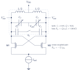
An LC tank stores energy and loses a little of it each cycle in the tank resistance. The cross-coupled pair of Figure 12.7 replaces that loss: looking into the two drains, the pair presents a negative resistance \(-2/g_\mathrm{m}\). The tank’s loss is a parallel resistance \(R_p = Q\omega_0 L\) (differential), so
Key equation · LC oscillator: frequency and start-up
\[f_0 = \frac{1}{2\pi\sqrt{L\,C_\mathrm{tot}}}, \qquad R_p = Q\,\omega_0 L, \qquad \text{oscillation if}\ \ \frac{g_\mathrm{m}R_p}{2} \ge 1 \ \ (\text{design for 2--3}). \tag{12.4}\]
The amplitude grows until the pair limits, at about \((4/\pi)\,I_\mathrm{tail}R_p/2\) (differential). \(C_\mathrm{tot}\) sums the varactors (fine tuning, which sets \(K_\mathrm{VCO}\)), a switched-capacitor bank (coarse bands for process corners) and all parasitics.
Worked Example 12.3 · The 2.5 GHz tank
Given: the team’s 4 nH differential inductor with \(Q = 16.8\) [9], \(f_0 = 2.5\) GHz. Capacitance: \(C_\mathrm{tot} = 1/(\omega_0^2L) = 1/\big((2\pi\cdot2.5\times10^9)^2\cdot4\times10^{-9}\big) = \mathbf{1.01}\) pF, including all parasitics. Loss: \(R_p = 16.8\times2\pi\cdot2.5\times10^9\times4\times10^{-9} = \mathbf{1.06}\) k\(\Omega\). Start-up: \(g_\mathrm{m}\ge 2/R_p = 1.89\) mS; with a 3\(\times\) margin, 5.7 mS per device (about 0.15 mA of collector current for an HBT, more for a MOSFET). Tuning: \(\pm10\%\) in frequency needs \(C_\mathrm{max}/C_\mathrm{min} = (1.1/0.9)^2 = 1.49\) across varactors and bank together, with the fixed parasitics counted in both.
Phase noise: Leeson’s model
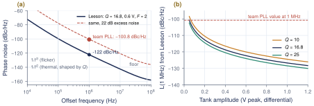
Leeson’s empirical model [38] captures the three regions of an oscillator’s phase noise (Figure 12.8a): \[\mathcal{L}(\Delta f) = 10\log_{10}\!\left[\frac{2FkT}{P_\mathrm{sig}}\left(1 + \Big(\frac{f_0}{2Q\,\Delta f}\Big)^2\right)\left(1 + \frac{f_{1/f^3}}{\Delta f}\right)\right] , \tag{12.5}\] where \(P_\mathrm{sig} = V_\mathrm{pk}^2/(2R_p)\) is the power in the tank and \(F\) an excess-noise factor of the active devices. Thermal noise near the carrier is shaped by the tank into a \(1/\Delta f^2\) slope, flicker noise adds \(1/\Delta f^3\) close in, and far out the noise is flat. For a fixed inductor, \(\mathcal{L} \propto 1/(Q\,V_\mathrm{pk}^2)\): a higher \(Q\) and a larger swing both help (Figure 12.8b).
Is \(-100.8\) dBc/Hz the VCO, or the PLL?
With \(Q = 16.8\), \(R_p = 1.06\) k\(\Omega\), 0.6 V of swing and \(F = 2\), Equation (12.5) predicts \(-122\) dBc/Hz at 1 MHz. The common oscillator figure of merit, \[\mathrm{FoM} = -\mathcal{L}(\Delta f) + 20\log_{10}(f_0/\Delta f) - 10\log_{10}(P/1\,\mathrm{mW}),\] would be only 162 dB for \(-100.8\) dBc/Hz at 5 mW of VCO power, against 180–190 dB for typical LC VCOs. The quoted value is probably the closed-loop PLL output near the loop bandwidth, or the VCO has excess noise (tail noise, low swing). This book uses it as free-running VCO noise, the pessimistic reading; resolving it is a Phase 0 task, because it moves the optimum of Worked Example 12.2.
Retuning the team’s 2.4 GHz design to 2.5 GHz
Keep the 4 nH inductor: its \(Q\) and layout are proven. The tank capacitance must fall from 1.10 to 1.01 pF, by 86 fF or 8%: remove one switched-capacitor unit or shift the band code, and re-check that \(V_\mathrm{ctrl}\) sits mid-range at all corners. \(R_p\) rises by 4% with frequency, so the start-up margin improves slightly. Replace the fractional-N divider with an integer \(\div50\) and redesign the loop filter for \(f_u \approx 3\) MHz (Worked Example 12.2). Target \(K_\mathrm{VCO}\approx 2\pi\times150\) MHz/V, so that supply and control noise stay small, and cover PVT with a 3–5 bit capacitor bank.
12.5Quadrature clocks and distribution
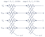
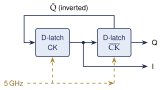
The half-rate receiver samples data on the 0\(^\circ\) and 180\(^\circ\) edges of the 2.5 GHz clock and the data transitions on the 90\(^\circ\) and 270\(^\circ\) edges, with four samplers D0, E0, D1, E1 (Section 10.2). It needs four phases, I, Q, \(\bar{\mathrm{I}}\) and \(\bar{\mathrm{Q}}\), spaced by exactly 100 ps. Open-SERDES derives them from the 2.5 GHz VCO with an RC polyphase filter (PPF); the alternative is a 5 GHz VCO followed by a \(\div2\) (Figure 12.9).
How accurate is the polyphase filter?
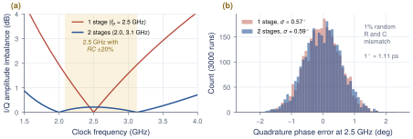
For a single stage driven differentially, the outputs are \(V/(1 + j\omega RC)\) and \(j\omega RC\,V/(1 + j\omega RC)\): always 90\(^\circ\) apart, with amplitude ratio \(\omega RC\). A \(\pm20\%\) process shift of \(RC\) therefore leaves 1.6–1.9 dB of amplitude imbalance, while two stages with poles at 2.0 and 3.1 GHz keep it below 0.07 dB (Figure 12.10a). Phase errors come from random mismatch instead: with 1% mismatch on every \(R\) and \(C\), Monte Carlo gives 0.57\(^\circ\) rms for one stage and 0.59\(^\circ\) for two (Figure 12.10b). The last stage sets the phase error, so it needs large, well-matched resistors and MIM capacitors in a common-centroid layout. The PPF is passive and lossy, \(-5.2\) dB for two unloaded stages, so CML buffers must restore the swing.
What the errors do to the half-rate samplers
At 2.5 GHz one degree is 1.11 ps. The CDR locks the edge samplers (Q, \(\bar{\mathrm{Q}}\)) onto the data transitions, so an I/Q error \(\delta\) moves the data samplers \(\delta\times1.11\) ps away from the eye centre: a static offset that eats timing margin. A duty-cycle error is worse, because the D1 and E1 samplers fire on the falling edges: a 1% duty error shifts them by 4 ps relative to D0 and E0, a two-valued DCD seen by every other bit.
Distribution
CML limiting buffers after the PPF restore the swing, remove the residual imbalance and keep the slew rate high (Equation (11.2)). Give them 2–3\(\times f_\mathrm{clk}\) of bandwidth (shunt peaking or tuned loads): a buffer near \(f_\mathrm{clk}\) amplifies jitter and duty-cycle error. A duty-cycle correction (DCC) loop that servoes the clock’s average to zero holds the duty cycle within about \(\pm0.5\%\).
Worked Example 12.4 · The RX clock-path line of the jitter budget
I/Q error: two-stage PPF, 1% mismatch: \(3\sigma = 3\times0.59^\circ = 1.8^\circ \to\) 2.0 ps. Duty cycle: \(\pm0.5\%\) after DCC: \(0.5\% \times 400\) ps \(\to\) 2.0 ps. PI nonlinearity: \(\pm0.6\) ps with corrected weights (Section 13.6) \(\to\) 1.2 ps. Total \(5.2\) ps, inside the 6 ps allocated in Table 11.1, with 0.8 ps of margin. Without DCC, a 52% duty cycle alone would cost 8 ps.
Open-SERDES clock generation targets
Integer-N CP-PLL, \(f_\mathrm{ref} = 50\) MHz, \(N = 50\), \(K_\mathrm{VCO}\approx 2\pi\times150\) MHz/V, \(I_\mathrm{CP}= 600\) A, \(f_u \approx 3\) MHz (\(f_{-3\mathrm{dB}} \approx 4.7\) MHz), 60\(^\circ\) phase margin. Jitter \(\le 1.0\) ps rms from 10 kHz and \(\le 0.6\) ps above 4 MHz. Quadrature from a two-stage PPF and CML buffers: I/Q error \(\le 2^\circ\) (\(3\sigma\)), duty cycle \(50 \pm 0.5\%\). Power estimate: PLL about 13 mW (the team’s design draws 12.73 mW); PPF buffers and distribution 10–15 mW (four CML stages of about 1.5 mA at 2.5 V).
Key takeaways
The PFD turns the edge offset into an UP/DN width difference; the charge pump gives \(I_\mathrm{CP}/2\pi\) A/rad. The reset delay removes the dead zone; current mismatch causes a static offset and reference spurs.
Type-II loop: \(\omega_n = \sqrt{I_\mathrm{CP}K_\mathrm{VCO}/(2\pi NC_1)}\), \(\zeta = (R/2)\sqrt{I_\mathrm{CP}K_\mathrm{VCO}C_1/(2\pi N)}\); peaking is 2.1 dB at \(\zeta = 0.707\) and 0.4 dB at \(\zeta = 2\).
For 60\(^\circ\) margin at 1 MHz: \(C_2\) = 4.07 pF, \(C_1\) = 52.6 pF, \(R\) = 11.3 k\(\Omega\) (\(f_{-3\mathrm{dB}}\) = 1.56 MHz); at the 3 MHz optimum, \(I_\mathrm{CP}\) = 600 A, \(C_1\) = 17.5 pF.
Reference noise is low-pass and VCO noise high-pass; the bandwidth that equalizes them, about 3 MHz here, minimizes jitter at 1.0 ps rms.
The 4 nH, \(Q = 16.8\) tank needs 1.01 pF at 2.5 GHz, has \(R_p\) = 1.06 k\(\Omega\), and oscillates if \(g_\mathrm{m}R_p/2 \ge 1\). Leeson suggests the quoted \(-100.8\) dBc/Hz is closed-loop: check it.
A two-stage PPF plus CML buffers gives I/Q within about 2\(^\circ\); every degree is 1.11 ps and every 1% of duty cycle is 4 ps at the half-rate samplers.
Generated from book/tutorial/chapters/12_pll.tex. Figure, table and equation numbers match the PDF edition.