Chapter 4Link Budgets and Statistical Analysis
The pulse response is enough to predict the eye: its worst case, its probability at \(10^{-12}\), and how much margin is left after noise, jitter and the sampler take their share.
In this chapter you will learn
Explain why superposition lets us predict every received sample from the cursors \(p_k\).
Derive the peak-distortion (worst-case) eye and the worst-case bit pattern, and apply them to REF.
Build a statistical eye by convolving ISI, noise and jitter distributions, and read eye height at \(10^{-12}\).
Write a top-down margin budget for the Open-SERDES receiver and decide what to spend margin on.
Decide between NRZ and PAM4 with the 9.54 dB rule.
4.1Pulse-response link analysis
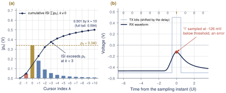
The channel, the TX FFE and the CTLE are linear and time-invariant, so the received waveform is a sum of shifted, scaled copies of one pulse response (Sections 2.3 and 2.4): \(y(t) = A\sum_n a_n\,p(t-nT_\mathrm{b})\). Sampling at \(t_\mathrm{s}+ nT_\mathrm{b}\) and writing \(p_k = p(t_\mathrm{s}+ kT_\mathrm{b})\) gives \[y_n = \underbrace{A\,a_n\,p_0}_{\text{signal}} \;+\; \underbrace{A\sum_{k\neq0} a_{n-k}\,p_k}_{\text{ISI}} \;+\; \text{noise}. \tag{4.1}\] At the sampler, the channel is a finite-impulse-response (FIR) filter whose taps are the cursors (Figure 4.1). Positive \(k\) are post-cursors, which come from earlier bits; negative \(k\) are pre-cursors, from later bits. Every question in this chapter (how bad the eye can get, how often, and how much margin is left) is answered from the list of \(p_k\), without simulating long bit streams.

4.2Peak distortion analysis
The worst case
Take a transmitted “1” (\(a_n = +1\)). By Equation (4.1), its sample is smallest when every ISI term pulls down, \(a_{n-k}\,p_k = -\lvert p_k\rvert\) for all \(k \ne 0\). The lowest “1” is then \(A(p_0 - \sum_{k\neq0}\lvert p_k\rvert)\), and by symmetry the highest “0” is its negative. The gap between them is the worst-case inner eye height.
Key equation · Peak-distortion eye and worst-case pattern
\[\mathrm{EH}(t_\mathrm{s}) = 2A\Big(p_0 - \sum_{k\neq0}\lvert p_k\rvert\Big), \qquad a_{n-k} = -\operatorname{sgn}(p_k)\,a_n . \tag{4.2}\]
This is peak distortion analysis (PDA) [13, 19]. It needs only the cursors, it bounds the eye for any bit stream, and the second half of Equation (4.2) gives the worst-case bit pattern. Because all cursors depend on the sampling instant, \(\mathrm{EH}\) is a function of \(t_\mathrm{s}\). Sweeping \(t_\mathrm{s}\) across the UI and keeping the range where \(\mathrm{EH}(t_\mathrm{s}) > 0\) gives the worst-case eye width.
Worked Example 4.1 · PDA of the REF channel
Given: the REF cursors of Table 3.2, \(2A = 1\) V, \(t_\mathrm{s}\) at the pulse peak.
Thirteen cursors: \(\sum_{k\neq0}\lvert p_k\rvert = 0.0486 + 0.1817 + 0.0909 + \cdots + 0.0084 = 0.501\) V, so \(\mathrm{EH} = 1\,\mathrm{V}\times(0.340 - 0.501) = \mathbf{-0.161\,V}\): closed. Figure 4.2(a) shows that the ISI already exceeds \(p_0\) after three post-cursors.
Full tail: the cursors beyond \(k = 10\) are small but many, and they add another 0.093 V. Summing out to 300 UI gives \(\mathrm{EH} = -0.255\) V. A check: all REF cursors are positive, so \(\sum_k p_k = H_\mathrm{ch}(0) = 0.935\) (the DC gain) and \(\mathrm{EH} = 2A(2p_0 - H_\mathrm{ch}(0)) = -0.255\) V.
Worst-case pattern: every \(p_k\) with \(k \neq 0\) is positive, so for \(a_n = +1\) all other bits are \(-1\): a lone “1” after a long run of “0”s, followed by a “0”. Figure 4.2(b) simulates it: the “1” arrives at \(-126\) mV, below the threshold.
PDA versus a PRBS simulation
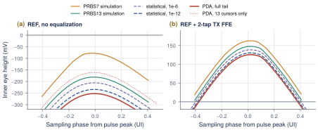
PDA is a bound, not a probability. The worst-case pattern for REF needs dozens of identical bits before the “1”; PRBS7 never has more than six “0”s in a row, so a PRBS7 simulation cannot find it. Figure 4.3 compares eye height versus sampling phase from PDA, from PRBS simulations and from the statistical eye of Section 4.3. On REF alone, PRBS7 reports \(-78\) mV (Section 16.3), PRBS13 \(-181\) mV and full-tail PDA \(-252\) mV: closed in every view. After a 2-tap TX de-emphasis, the ranking is the same: PRBS7 163 mV, PRBS13 148 mV, PDA 126 mV. A short PRBS is optimistic because it never visits the rare patterns that set the eye at \(10^{-12}\).
Truncating the tail
PDA sums \(\lvert p_k\rvert\) over all \(k\). Many small cursors add up: for REF, the cursors beyond \(k = 10\) are each below 0.008 V yet add 0.093 V. Always extend the cursor list until the tail is negligible, and simulate with a PRBS whose period is longer than the channel memory (PRBS13 or longer for REF), or the eye will look better than it is.
4.3The statistical eye
PDA tells us the worst case but not how often it happens. A BER target is a statement about probability, so we want the distribution of \(y_n\). In Equation (4.1) each ISI term \(A\,a_{n-k}p_k\) is an independent random variable that takes \(+A p_k\) or \(-A p_k\) with probability \(\tfrac12\). The PDF of a sum of independent variables is the convolution of their PDFs, so the ISI PDF is built one cursor at a time (Figure 4.4a): one cursor gives two spikes, two give four, \(m\) give up to \(2^m\), and the shape fills in [19, 20].
Key equation · Statistical eye
\[\begin{gather} f_\mathrm{ISI}(v) = \mathop{\large \ast}_{k\neq0}\Big[\tfrac12\delta(v - A p_k) + \tfrac12\delta(v + A p_k)\Big], \qquad f_X = f_\mathrm{ISI} \ast \mathcal N(0,\sigma_\mathrm{n}^2), \tag{4.3}\\ \mathrm{BER}(t_\mathrm{s}, v) = \tfrac12 P(A p_0 + X < v) + \tfrac12 P(-A p_0 + X > v), \tag{4.4}\\ \mathrm{BER}_J(t_\mathrm{s}, v) = \int \mathrm{BER}(t_\mathrm{s}- \tau, v)\, f_J(\tau)\,d\tau . \tag{4.5} \end{gather}\]
Gaussian noise of rms \(\sigma_\mathrm{n}\) is one more convolution in voltage. Sampling-clock jitter moves \(t_\mathrm{s}\), so it is a convolution in time with the jitter PDF \(f_J\). Here we use the dual-Dirac model [21] (a Gaussian of rms \(\sigma_\mathrm{RJ}\) at \(\pm\mathrm{DJ}/2\)); Section 11.3 explains where it comes from. Evaluating Equation (4.4) over a grid of \((t_\mathrm{s}, v)\) gives the statistical eye: contours of constant BER. The vertical bathtub is one column of it, BER versus threshold at a fixed phase. The eye height at a BER target is the width of the bathtub at that BER.
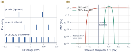
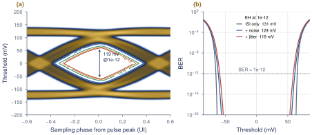
The statistical eye needs a channel that is open, so from here on we use REF with the 2-tap TX de-emphasis of Lab 3, \(c_0 = 0.652\) and \(c_1 = -0.348\) (Sections 6.2 and 16.4). It is the simplest equalizer that opens REF, not the final Open-SERDES design. Figure 4.5 shows its statistical eye with noise and jitter. The code is stat_eye() in figsrc/ch04_stateye.py: a few dozen lines of NumPy that shift and add the two-point PDFs on a 0.05 mV grid.
Worked Example 4.2 · PDA versus statistical eye height
Given: REF with 2-tap de-emphasis. The equalized pulse peaks at \(q_0 = 0.209\) V, 22 ps earlier than REF. Its residual cursors are \(q_{-1} = 0.0155\), \(q_1 = 0.0125\), \(q_2 = -0.0056\), then a slowly decaying tail of 0.002–0.0045 V per UI. \(\sum_{k\neq0}\lvert q_k\rvert = 0.084\) V.
PDA: \(\mathrm{EH} = 1\,\mathrm{V}\times(0.209 - 0.084) = \mathbf{126}\) mV, open over 0.75 UI.
Statistical eye, ISI only: 139 mV at \(10^{-6}\) and 131 mV at \(10^{-12}\), open over 0.77 UI.
With noise and jitter: \(\sigma_\mathrm{n}= 1.5\) mV gives 123 mV; adding 2 ps RJ and 20 ps DJ gives 119 mV and cuts the width to 0.59 UI.
Interpretation: at \(10^{-12}\) the statistical eye is only 4% larger than PDA. A probability of \(10^{-12} \approx 2^{-40}\) means roughly 40 cursors line up in their worst direction, and here the cursors beyond the first 40 add only 0.006 V. PDA is far too pessimistic only when the ISI is spread over many comparable cursors. A large gap between PDA and the statistical eye should make you check your tail, not celebrate.
What this means for your design
Use the three tools for different jobs. PDA is instant and gives the worst-case pattern, which is the best stimulus for a transistor-level simulation. The statistical eye answers the actual specification, eye height and width at \(10^{-12}\), and is where noise and jitter enter. A PRBS7 eye from a short transient is a sanity check, never a sign-off. For REF-like channels, PDA is within a few percent of the \(10^{-12}\) eye, so design to PDA early and confirm with the statistical eye.
Statistical eye in serdespy
Import stat_eye and eye_metrics from ch04_stateye.py, and feed them the pulse response from any lab (Sections 16.3 and 16.4). Change sigma_n, rj and dj and watch which one moves the height and which the width.
4.4The system noise and margin budget
A margin budget starts from the transmitted swing and subtracts, step by step, everything that eats the eye before the sampler decides. Whatever is left is the margin that covers what the model does not know: process corners, crosstalk, adaptation error. The terms are:
TX swing \(2A\) = 1 Vppd.
Channel loss, which shrinks the main cursor to \(2A p_0\).
Equalization: a TX FFE costs main cursor (Chapter 6); a CTLE and DFE do not, to first order.
Residual ISI at the BER target, from the statistical eye.
RX noise: for Gaussian noise of rms \(\sigma_\mathrm{n}\), a BER of \(10^{-12}\) needs \(\mathrm{EH} \ge 2Q\sigma_\mathrm{n}= 14.07\,\sigma_\mathrm{n}\) (Equation (2.9)).
Jitter: sampling away from the best phase lowers the eye.
Sampler offset \(V_\mathrm{os}\) and sensitivity \(V_\mathrm{sens}\) (Sections 10.4 and 10.2).
Key equation · Linear margin budget at the sampler
\[M = \mathrm{EH}_\mathrm{ISI}(10^{-12}) - 2Q\,\sigma_\mathrm{n}- \Delta V_\mathrm{jitter} - 2V_\mathrm{os} - V_\mathrm{sens} \;>\; 0 . \tag{4.6}\]
An offset moves the threshold toward one rail, so the worse half-eye shrinks by \(V_\mathrm{os}\); that costs \(2V_\mathrm{os}\) of symmetric eye height. The sensitivity is the minimum peak-to-peak input the sampler resolves in time. All terms are referred to the RX input.
Worked Example 4.3 · Margin budget for REF with 2-tap de-emphasis
Assumptions: \(\sigma_\mathrm{n}= 1.5\) mV rms input-referred (CTLE plus samplers); sampling jitter of 2 ps RJ and 20 ps DJ, the latter from PI quantization dither (6.25 ps steps) and CDR wander (Section 11.5); offset after calibration \(V_\mathrm{os} = 5\) mV; sampler sensitivity \(V_\mathrm{sens} = 20\) mV.
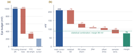
Stack-up (Figure 4.6): 1000 mV \(\to\) channel \(\to\) 340 mV main cursor \(\to\) de-emphasis \(\to\) 209 mV \(\to\) residual ISI at \(10^{-12}\) \(\to\) 131 mV. Then noise \(2Q\sigma_\mathrm{n}= 14.07\times1.5 = 21\) mV, jitter 3.5 mV, offset \(2\times5 = 10\) mV and sensitivity 20 mV leave \(M \approx 76\) mV.
Statistical check: the statistical eye with noise and jitter included is 119 mV, which leaves \(119 - 10 - 20 = 89\) mV. Noise really costs only 8 mV here, not 21 mV, because the \(7\sigma\) noise peak rarely coincides with a worst-case ISI pattern. The linear budget is conservative by 13 mV.
What to spend margin on
The largest term is residual ISI (79 mV), not noise (8–21 mV). The best use of design effort is therefore equalization: the CTLE and 2-tap DFE of Chapters 7 and 8 remove most of the residual ISI without the main-cursor cost of a TX FFE (Section 8.5). Keep the margin for things the model leaves out: the 20–25 dB end of LOSS_FAMILY (each extra dB of Nyquist loss shrinks the main cursor by about 6%), crosstalk (25 mVpp of NEXT would take a third of it), termination and CTLE drift over corners, and DFE tap error. Do not spend power to push \(\sigma_\mathrm{n}\) below 1 mV: halving it buys only a few millivolts.
4.5Modulation choice: NRZ or PAM4?
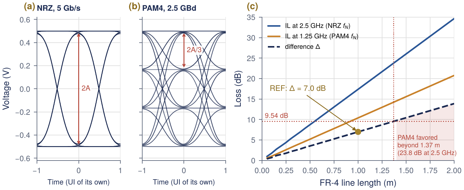
PAM4 sends two bits per symbol on four levels, \(\{-A, -A/3, +A/3, +A\}\). At the same bit rate the symbol rate halves (2.5 GBd for 5 Gb/s), so the Nyquist frequency halves to 1.25 GHz and the channel loss there is smaller. The price is that the three stacked eyes are each \(2A/3\) high instead of \(2A\) (Figure 4.7a,b).
Key equation · The PAM4 rule
\[20\log_{10}3 = 9.54\,\mathrm{dB} \qquad\Longrightarrow\qquad \text{PAM4 wins only if}\quad \Delta = \mathrm{IL}(f_\mathrm{N}) - \mathrm{IL}(f_\mathrm{N}/2) > 9.54\,\mathrm{dB}. \tag{4.7}\]
PAM4 recovers its 9.54 dB eye penalty only if the channel loses more than that between the two Nyquist frequencies, which are an octave apart. If the loss were proportional to \(f\) (pure dielectric), \(\Delta\) would be half the NRZ Nyquist loss; if it were proportional to \(\sqrt f\) (pure skin effect), \(\Delta = 0.29\,\mathrm{IL}(f_\mathrm{N})\). Real FR-4 sits in between.
Worked Example 4.4 · NRZ or PAM4 for Open-SERDES?
Given: channel() from link.py for REF and the LOSS_FAMILY lengths.
Solution: Table 4.1 lists the losses at both Nyquist frequencies. For our model \(\Delta \approx 0.40\,\mathrm{IL}(f_\mathrm{N})\). REF has \(\Delta = 17.4 - 10.4 = 7.0\) dB, so NRZ wins by \(9.54 - 7.0 = 2.6\) dB. \(\Delta\) reaches 9.54 dB at 1.37 m, where the NRZ Nyquist loss is 23.8 dB (Figure 4.7c). Only the 25 and 30 dB channels pass the rule, and only by 0.5 and 2.5 dB.
| Channel | Length (m) | IL at 2.5 GHz (dB) | IL at 1.25 GHz (dB) | \(\Delta\) (dB) | Rule favors |
|---|---|---|---|---|---|
| 5 dB | 0.285 | 5.0 | 3.0 | 2.0 | NRZ |
| 10 dB | 0.572 | 10.0 | 6.0 | 4.0 | NRZ |
| 15 dB | 0.862 | 15.0 | 9.0 | 6.0 | NRZ |
| REF | 1.000 | 17.4 | 10.4 | 7.0 | NRZ |
| 20 dB | 1.152 | 20.0 | 12.0 | 8.0 | NRZ |
| 25 dB | 1.441 | 25.0 | 15.0 | 10.0 | PAM4 (barely) |
| 30 dB | 1.731 | 30.0 | 18.0 | 12.0 | PAM4 |
The rule is a first-order comparison, and it flatters PAM4. A DFE cancels post-cursors for either format, but whatever ISI is left (pre-cursors, tap errors) weighs three times more against a PAM4 eye. PAM4 also needs three comparators per sampling phase (up to twelve samplers instead of the two data and two edge samplers of our half-rate receiver), reference levels that track the signal amplitude, a linear TX driver and CTLE, and a CDR that copes with several zero-crossing times per transition. It is also three times more sensitive to residual ISI, crosstalk and sampler offset.
Open-SERDES decision
Open-SERDES uses NRZ. Over REF and every channel up to 20 dB, NRZ wins by the 9.54 dB rule, and it costs a third of the slicers. PAM4 is kept as a Phase-4 option, worth revisiting only for channels beyond about 24 dB at 2.5 GHz or for a 10 Gb/s follow-on (Table 14.4).
4.6Exercises
PDA by hand. A channel has \(p_{-1} = 0.05\), \(p_0 = 0.50\), \(p_1 = 0.20\), \(p_2 = -0.04\), \(p_3 = 0.02\). Find the PDA eye for \(2A = 0.8\) V and the worst-case bit pattern in time order.
The tail matters. Using
link.cursorswithn_post= 10, 30, 100 and 300, plot the REF PDA eye againstn_post. How many cursors do you need before the answer changes by less than 5 mV?Two cursors, exactly. For ISI from only \(p_1\) and \(p_2\), write the ISI PDF and the BER versus threshold in closed form, with Gaussian noise \(\sigma_\mathrm{n}\). Compare with
stat_eye().Budget. Redo Worked Example 4.3 with \(\sigma_\mathrm{n}= 3\) mV and an uncalibrated offset of 15 mV. Is the margin still positive? Which single improvement restores the most margin?
PAM4 at 10 Gb/s. For a 10 Gb/s follow-on over REF, compare NRZ (\(f_\mathrm{N}= 5\) GHz) with PAM4 (\(f_\mathrm{N}= 2.5\) GHz) using
loss_db. Which wins by the rule?
Key takeaways
At the sampler, the channel is an FIR filter with taps \(p_k\), so the cursors alone predict every received sample.
PDA gives the worst-case eye \(2A(p_0 - \sum_{k\neq0}\lvert p_k\rvert)\) and the worst-case pattern \(a_{n-k} = -\operatorname{sgn}(p_k)\,a_n\). REF is closed: \(-0.161\) V with 13 cursors, \(-0.255\) V with the full tail.
The statistical eye convolves two-point ISI distributions with noise (in voltage) and jitter (in time) to give BER contours. For REF with 2-tap de-emphasis: PDA 126 mV, statistical 131 mV at \(10^{-12}\), 119 mV with noise and jitter.
Short PRBS simulations are optimistic (PRBS7: 163 mV) because they never meet the rare worst-case patterns.
A linear margin budget for that link leaves about 76 mV (89 mV statistically). Residual ISI, not noise, is the largest term, so spend design effort on equalization.
PAM4 pays 9.54 dB of eye height and wins only if the loss between 1.25 and 2.5 GHz exceeds that. REF has 7.0 dB, so Open-SERDES uses NRZ.
Generated from book/tutorial/chapters/04_linkanalysis.tex. Figure, table and equation numbers match the PDF edition.