Chapter 13Clock and Data Recovery
The receiver has no clock wire: it must find the centre of every bit from the data itself, and keep finding it while the two crystals drift apart.
In this chapter you will learn
Explain why a receiver needs a CDR and compare PLL-based, PI-based and oversampling architectures.
Analyze the Hogge (linear) and Alexander (bang-bang) phase detectors, including the half-rate version used by Open-SERDES.
Model a linear CDR and a bang-bang CDR: gain \(K_\mathrm{BB}\), slewing bandwidth and dither.
Read a jitter-tolerance mask and size the loop to pass it.
Design the Open-SERDES phase-interpolator CDR: PI linearity, step size, frequency-offset range and a behavioural simulation.
13.1Why the receiver needs a CDR
The TX and RX of a serial link run from different crystals, each accurate to about \(\pm100\) ppm. Their bit rates can differ by 200 ppm, so the data phase drifts past a fixed RX clock by \(2\times10^{-4}\) UI every UI: one whole UI every 5000 bits, or every microsecond at 5 Gb/s. A fixed-phase sampler would walk out of the eye within half a microsecond, so the receiver must extract phase and frequency from the data transitions: clock and data recovery (CDR). Line coding or scrambling guarantees the transitions, and the CDR tracks slow jitter as a bonus (Section 11.6).
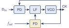
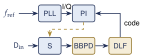
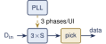
Figure 13.1 shows the three common architectures. A PLL-based CDR has a VCO in the loop: lowest dither, but a VCO per lane and a frequency detector to pull in. A PI-based dual-loop CDR shares one clean PLL and rotates its phase per lane with a digitally controlled phase interpolator: synthesizable, free of false lock and robust over PVT, at the cost of quantization and latency. An oversampling CDR samples three times per UI and picks the best sample, with no loop but three times the samplers. Open-SERDES uses the PI dual loop because it reuses the team’s PLL (Chapter 12).
13.2Phase detectors
A PLL’s PFD does not work on data: random data skips edges, and a missing edge looks like a frequency error. A CDR phase detector must compare edges only where the data has them, and output nothing during runs of identical bits (tri-state). Two classic detectors do this.
The Hogge linear detector
Hogge’s detector [39] uses two flip-flops and two XORs (Figure 13.2). FF1 retimes the data (B), FF2 delays B by half a cycle (A). \(X = D_\mathrm{in}\oplus B\) lasts from each data transition to the next rising clock edge, \(T_\mathrm{b}/2 + \Delta t\) when the clock is \(\Delta t\) late; \(Y = B\oplus A\) always lasts \(T_\mathrm{b}/2\). X pumps up and Y pumps down, so the net charge per transition is proportional to \(\Delta t\): a linear detector of gain \(TD\cdot I_P/2\pi\), where the transition density TD is about 0.5 for random data. It tri-states and retimes the data. Its weakness is speed: at 5 Gb/s X and Y are 100 ps pulses from gates with 20–30 ps edges, and the clock-to-Q delay leaves a static error unless matched; at 10 Gb/s the pulses shrink to 50 ps, close to the practical limit.
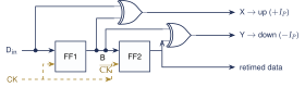
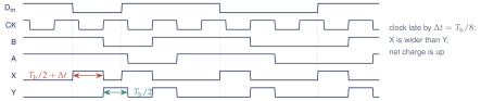
After Razavi [40].
The Alexander bang-bang detector
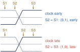
The Alexander detector [41] (Figure 13.3) takes two samples per bit: a data sample at the bit centre and an edge sample half a bit earlier, at the expected transition. Three consecutive samples, S1 (previous data), S2 (edge) and S3 (current data), tell everything. If S1 = S3 there was no transition and the detector says nothing. Otherwise S2 equals whichever data bit it was closer to: if S2 = S1 the edge sample was taken before the transition and the clock is early; if S2 = S3 it was taken after, and the clock is late. With \(X = S1\oplus S2\) and \(Y = S2\oplus S3\):
| \((X, Y)\) | (0,0) | (0,1) | (1,0) |
|---|---|---|---|
| Meaning | no transition | clock early: delay it | clock late: advance it |
The output is only the sign of the error, hence “bang-bang” (BB). It reuses the data samplers, retimes, tri-states and runs at the samplers’ full speed: the most common CDR detector.
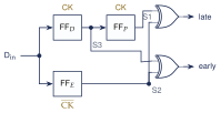
Half-rate in Open-SERDES
At half rate the four samplers D0, E0, D1, E1 fire on I, Q, \(\bar{\mathrm{I}}\), \(\bar{\mathrm{Q}}\) of the 2.5 GHz clock (Sections 12.5 and 10.2). Each clock cycle yields two early/late decisions, from (D0, E0, D1) and (D1, E1, D0\('\)), so every transition is used. The cost is that I/Q and duty-cycle errors now appear as phase offsets between the two halves (Worked Example 12.4).
Mueller-Müller
This baud-rate detector [42] uses one data sample and one error sample per UI and no edge samplers. Its output \(z_k = e_k d_{k-1} - e_{k-1}d_k\) averages to \(h_1 - h_{-1}\), so it locks where the first pre- and post-cursors are equal, a channel-dependent point. It suits ADC-based receivers; Open-SERDES has edge samplers and uses Alexander.
13.3The linear CDR model and jitter transfer
With a linear detector, a CDR is a PLL with \(N = 1\) and a detector gain \(TD\cdot I_P/2\pi\). With proportional resistor \(R_p\) and integrating capacitor \(C_p\), Equation (12.1) gives
Key equation · Linear CDR
\[\begin{gathered} H(s) = \frac{\phi_\mathrm{out}}{\phi_\mathrm{in}} = \frac{2\zeta\omega_n s + \omega_n^2}{s^2 + 2\zeta\omega_n s + \omega_n^2}, \\ \omega_n = \sqrt{\frac{K_\mathrm{VCO}I_P}{2\pi C_p}}, \qquad \zeta = \frac{R_p}{2}\sqrt{\frac{K_\mathrm{VCO}I_P C_p}{2\pi}}, \qquad \omega_{-3\mathrm{dB}} \approx 2\zeta\omega_n = \frac{K_\mathrm{VCO}I_P R_p}{2\pi} . \end{gathered} \tag{13.1}\]
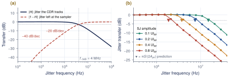
with TD absorbed into \(I_P\). \(|H|\) is the jitter transfer: the jitter the recovered clock follows. \(|1 - H|\) is what the clock does not follow, and therefore what reaches the sampler as eye closure (Figure 13.4a). Wireline CDRs use \(\zeta \gg 1\), typically 4–5, because any peaking would amplify jitter in a chain of repeaters; with \(\zeta = 4.5\) the peaking is 0.09 dB (Table 12.1).
13.4Bang-bang CDR dynamics
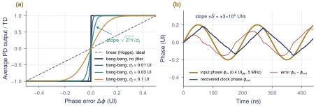
A BB detector has infinite gain at zero error, but jitter rescues the linear model: with Gaussian edge jitter of rms \(\sigma_j\), the average output is the sign function smoothed by the jitter PDF: \[\overline{\mathrm{PD}}(\Delta\phi) = TD\cdot E\big[\operatorname{sgn}(\Delta\phi + j)\big] = TD\cdot\operatorname{erf}\!\Big(\frac{\Delta\phi}{\sqrt2\,\sigma_j}\Big),\] whose slope at zero, \(TD\cdot 2/(\sqrt{2\pi}\sigma_j)\), is the linearized gain (Figure 13.5a):
Key equation · Bang-bang detector gain, linearized by jitter
\[K_\mathrm{BB} = TD\,\sqrt{\frac{2}{\pi}}\,\frac{1}{\sigma_j} \quad \text{(per UI of phase error)} . \tag{13.2}\]
The loop gain, and so the bandwidth, is inversely proportional to the input jitter: a clean input makes a fast loop, a noisy input a slow one. Always quote a BB-CDR’s bandwidth together with the jitter it was measured with.
Slewing
For large jitter the detector saturates and the recovered phase moves at its maximum rate, the slew rate \(S\). In a VCO-based loop each decision shifts the VCO frequency by \(\Delta f_P = K_\mathrm{VCO}I_P R_p\) for one bit, moving the phase by \(\Delta\phi_P = \Delta f_P\,T_\mathrm{b}\) clock cycles, and decisions arrive at rate \(TD/T_\mathrm{b}\); so \(S = TD\,\Delta\phi_P/T_\mathrm{b}\). A sinusoid \(A_\mathrm{pk}\sin\omega t\) is tracked as long as its peak slope \(\omega A_\mathrm{pk}\) is below \(S\). Beyond that the output is a triangle of peak \(S\,T/4\) (Figure 13.5b), so its gain is \(\pi S/(2A_\mathrm{pk}\omega)\) and
Key equation · Slew-limited BB-CDR bandwidth
\[S = TD\,\frac{\Delta\phi_P}{T_\mathrm{b}}, \qquad \omega_{-3\mathrm{dB}} = \frac{\pi S}{2A_\mathrm{pk}}, \qquad \text{dither}_\mathrm{pp} \approx 2(D+1)\,\Delta\phi_P . \tag{13.3}\]
The last term is the dither: with no jitter at all, a BB loop hunts around the lock point, and a loop latency of \(D\) extra decision periods lets it overshoot by \(D\) more steps each way. Large \(S\) helps jitter tolerance but costs dither; the integral path must be weak compared with the proportional path, \(K_P/K_I \ge 16\) (for an analog loop, \(R_pC_p/T_\mathrm{b}\gg 1\)), or the loop rings.
| Jitter (UI\(_\mathrm{pp}\)) | 0.125 | 0.25 | 0.5 | \(R_p\) (\(\Omega\)) / \(C_p\) (nF) | 5 / 100 | 10 / 100 | 20 / 100 |
| Predicted \(f_{-3\mathrm{dB}}\) (MHz) | 6.0 | 3.0 | 1.5 | Measured (MHz) | 1.0 | 1.5 | 2.7 |
| Measured (MHz) | 4.1 | 2.8 | 1.45 | \(C_p\) = 10 / 32 / 100 nF | 2.8 / 2.55 / 2.6 | ||
Table 13.1 checks Equation (13.3) against measurements. The prediction matches at 0.25 and 0.5 UI\(_\mathrm{pp}\); at 0.125 UI the loop is no longer slewing (the input slope is below \(S\)) and the measured corner saturates. The bandwidth scales with \(R_p\), the proportional path, and hardly depends on \(C_p\): a BB-CDR is designed through its proportional step.
Worked Example 13.1 · An analog BB-CDR that fails, and the fix
Given: a half-rate VCO-based BB-CDR at 5 Gb/s, \(K_\mathrm{VCO}\) = 150 MHz/V, \(I_P\) = 100 A, \(R_p\) = 100 \(\Omega\), \(C_p\) = 1 nF, \(TD\) = 0.5, and a stressed input that leaves a timing margin TM = 0.4 UI.
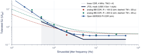
Step: \(\Delta f_P\) = 1.5 MHz; one cycle of the 2.5 GHz clock is 2 UI, so \(\Delta\phi_P = 1.5\times10^6\times200\,\mathrm{ps}\times2 = 6\times10^{-4}\) UI per bit and \(S = 0.5\times6\times10^{-4}/200\,\mathrm{ps} = 1.5\times10^6\) UI/s. JTOL (Section 13.5): \(\mathrm{TM} + 2S/\omega = 0.4 + 0.48 = 0.88\) UI\(_\mathrm{pp}\) at 1 MHz, below the 1 UI mask point: fails. Simulation gives 0.95 UI at 1 MHz and 0.35 UI at 2 MHz (mask 0.5). Fix: \(R_p\) = 200 \(\Omega\) doubles \(S\) to \(3\times10^6\) UI/s: \(0.4 + 0.95 = 1.35\) UI at 1 MHz (simulated 1.36) and 0.61 UI at 2 MHz: passes. Costs: dither with a 3-bit latency is \(2\times4\times1.2\times10^{-3} = 0.01\) UI, negligible. \(R_pC_p/T_\mathrm{b}= 1000\), so the loop is well damped. The proportional path alone pulls in only \(|\Delta f/f| < TD\,\Delta\phi_P \approx 600\) ppm, so a frequency detector or reference loop must bring the VCO that close first.
13.5Jitter tolerance
Jitter tolerance (JTOL) is the largest sinusoidal jitter (SJ), versus frequency, that the receiver accepts while meeting the BER, measured with a stressed input that already carries the specified RJ and DJ. Let TM be the timing margin left by that stress. A linear CDR leaves the error \(|1-H|\) times the input, so \[\mathrm{JTOL}(\omega) = \frac{\mathrm{TM}}{|1 - H(j\omega)|}, \qquad \mathrm{JTOL}_\mathrm{BB}(\omega) \approx \mathrm{TM} + \frac{2S}{\omega} . \tag{13.4}\] Far below the bandwidth the CDR tracks almost everything and JTOL is many UI; far above, JTOL falls to TM. A BB-CDR in its slew-limited region follows \(2S/\omega\), a \(-20\) dB/decade line. Standards define a JTOL mask that the curve must stay above. We use a USB 3 Gen 1-style mask: 2 UI\(_\mathrm{pp}\) at 0.5 MHz falling at \(-20\) dB/decade to 0.2 UI at 4.9 MHz, flat to 50 MHz (check the exact points against the standard you target). Passing the \(-20\) dB/decade part needs \(S \gtrsim \pi f(A_\mathrm{mask} - \mathrm{TM})\), about \(2.5\times10^6\) UI/s at 0.5 MHz.
13.6The Open-SERDES PI-based CDR
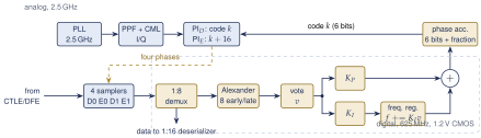
Figure 13.7 shows the Open-SERDES CDR. The PLL supplies I and Q at 2.5 GHz. Two phase interpolators (PIs) rotate them: the data PI (code \(k\)) clocks D0 and D1, the edge PI (code \(k + 16\), a quarter period later) clocks E0 and E1. A 1:8 demultiplexer feeds the digital loop at 625 MHz (\(T_\mathrm{upd}\) = 1.6 ns, 8 UI), where up to eight Alexander early/late decisions per update are reduced by a majority vote to \(v \in \{-1, 0, +1\}\). The loop filter is proportional plus integral: \[f \leftarrow f + K_I\,v, \qquad \mathrm{acc} \leftarrow \mathrm{acc} + K_P\,v + f, \qquad k = \mathrm{round}(\mathrm{acc}) \bmod 64 .\] The frequency register \(f\) learns the TX-RX frequency offset, and the phase accumulator has fractional bits below the PI’s 6.25 ps LSB, so the proportional step \(K_P\) can be a fraction of a PI step. The baseline uses \(K_P = 1/8\) LSB (0.78 ps), \(K_P/K_I = 128\) and a latency of two updates (\(D = 1\)).
The phase interpolator
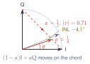
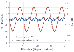
A PI forms \((1-\alpha)\,\mathrm{I} + \alpha\,\mathrm{Q}\) with two current-steered weights. For sinusoidal I and Q the output phase is \(\theta = \arctan[\alpha/(1-\alpha)]\), not \(90^\circ\alpha\): linear weights trace the chord between the two phasors, not the arc (Figure 13.8a). With 16 codes per quadrant, the integral nonlinearity (INL) reaches \(\pm4.1^\circ\) (\(\pm4.5\) ps) at \(\alpha \approx 0.25\) and 0.75, and the amplitude dips to 0.71 at \(\alpha = 0.5\). Weights taken from a sine/cosine table and quantized to 6 bits cut the INL to \(\pm0.55^\circ\) (0.6 ps) (Figure 13.8b); a limiting buffer after the PI removes the amplitude dip. The law assumes near-sinusoidal inputs, with edges about as slow as the 100 ps phase spacing, which the PPF and CML buffers of Section 12.5 provide; square-wave inputs make the PI jump between phases.
Frequency-offset range
A \(\pm300\) ppm offset (two \(\pm100\) ppm crystals plus margin) drifts the data by \(300\times10^{-6}\times1.6\,\mathrm{ns} = 0.48\) ps per update, 0.077 PI step; the integral register holds this rate and the PI rotates continuously, wrapping every 833 updates (1.33 s). The proportional path alone could follow \(0.78\,\mathrm{ps}/1.6\,\mathrm{ns} = 488\) ppm, so \(\pm300\) ppm would use 61% of its slew: hence the integral path. The PI’s ceiling, one step per update, is \(6.25\,\mathrm{ps}/1.6\,\mathrm{ns} = 3906\) ppm. The rotating code sweeps the INL pattern at four times the 750 kHz rotation rate, a 3 MHz periodic jitter. Spread-spectrum clocking (5000 ppm) is out of range.
Worked Example 13.2 · PI step size: 64 or 128 steps?
Question: does doubling the PI resolution reduce the CDR’s own jitter? Method: the behavioural model of ch13_sim.py: +200 ppm offset, input RJ 1.32 ps and \(\pm10\) ps DDJ, \(K_P\) chosen so that every design has the same slew \(S = 2.44\times10^6\) UI/s (the JTOL requirement), \(D\) = 1. “Wander” is the recovered-phase error; the peak-to-peak value is taken at the \(10^{-5}\) quantiles of \(1.2\times10^5\) updates.
| PI steps | loop clock | \(K_P\) | wander rms | wander pp | JTOL vs mask |
|---|---|---|---|---|---|
| 64 | 312.5 MHz | 1 LSB (integer) | 10.7 ps | 58.1 ps | 2.6\(\times\) |
| 64 | 312.5 MHz | 1/4 LSB | 3.3 ps | 24.3 ps | pass |
| 128 | 312.5 MHz | 1/2 LSB | 2.9 ps | 23.0 ps | pass |
| 64 | 625 MHz | 1/8 LSB | 2.5 ps | 19.2 ps | pass |
| 128 | 625 MHz | 1/4 LSB | 1.9 ps | 15.6 ps | pass |
Answer: at a fixed loop clock, 128 steps saves only 1.3 ps. What matters is the proportional step in picoseconds (fixed by JTOL) and the latency in nanoseconds, since dither \(\approx 2S\,T_\mathrm{lat}\); an integer-step loop is far too noisy. A 625 MHz loop halves the latency and brings 64 steps inside the 20 ps allocation of Table 11.1. Keep 64 steps; use 128 only if the 625 MHz loop fails timing.
Behavioural check
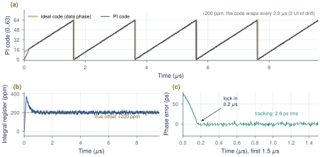
In Figure 13.9 the baseline starts 0.37 UI off with +200 ppm offset: it locks in 0.19 s, the integral register settles at 200 ppm within about 1 s, and the tracking error is 2.6 ps rms. The same model gives the JTOL curve in Figure 13.6: 3.0 UI\(_\mathrm{pp}\) at 0.5 MHz, 1.08 at 1 MHz, 0.51 at 2 MHz (mask 0.5: marginal, within the sweep’s 10% resolution) and 0.32 at high frequency. Its jitter transfer has a \(-3\) dB corner near 9 MHz for 0.2 UI\(_\mathrm{pp}\) input and 16 MHz for 0.05 UI\(_\mathrm{pp}\), as Equation (13.3) predicts for a BB loop; Chapter 11 conservatively assumed 4 MHz when counting the PLL’s untracked jitter.
What this means for your design
Size a BB-CDR in this order: \(S\) from the JTOL mask; \(K_P\cdot\mathrm{LSB} = S\,T_\mathrm{upd}\); the shortest latency the logic allows (dither \(\propto S\,T_\mathrm{lat}\)); then \(K_I \le K_P/16\) and an integral register wide enough for the ppm range.
Lab 7: CDR
Section 16.8 builds a fuller version of ch13_sim.py. Reproduce Figure 13.9, then sweep \(K_P\) and the latency \(D\) and plot wander against JTOL margin: you will find the trade-off of Worked Example 13.2.
Open-SERDES CDR targets
Half-rate Alexander BBPD; two 64-step PIs (6.25 ps) with sine/cosine weights (INL \(\le 1^\circ\)); P+I loop at 625 MHz, \(K_P\) = 1/8 LSB, \(K_P/K_I\) = 128, latency \(\le\) 2 updates; \(\pm300\) ppm; lock \(<\) 1 s; wander \(\le\) 20 ps pp; JTOL above the mask with TM = 0.4 UI. Power estimate: PIs and buffers 6–10 mW, digital loop about 2 mW.
13.7Exercises
TX and RX crystals are at \(+100\) and \(-80\) ppm. How long does the data take to drift one UI at 5 Gb/s, and how many PI codes per microsecond must the CDR rotate?
In the Hogge detector at 5 Gb/s, the clock is 20 ps early. Give the widths of X and Y, and the average current for \(I_P\) = 100 A and \(TD\) = 0.5.
A BB-CDR sees \(\sigma_j\) = 0.03 UI. Compute \(K_\mathrm{BB}\) for \(TD\) = 0.5. By what factor does the small-signal bandwidth change if the channel doubles the jitter?
For a 625 MHz loop, find the smallest \(K_P\) (in PI LSBs) that passes the mask point 2 UI\(_\mathrm{pp}\) at 0.5 MHz with TM = 0.4 UI. What dither would \(D = 3\) give?
Key takeaways
200 ppm drifts one UI per microsecond, so the receiver recovers phase and frequency from the data; Open-SERDES uses a PI dual loop that reuses the PLL.
Hogge is linear but needs 100 ps pulses; Alexander reuses the samplers: (0,1) early, (1,0) late, (0,0) no transition.
Linear CDR: a PLL with \(N = 1\), \(\omega_{-3\mathrm{dB}} \approx K_\mathrm{VCO}I_P R_p/2\pi\); only \(|1-H|\) of the jitter reaches the sampler.
Bang-bang: \(K_\mathrm{BB} = TD\sqrt{2/\pi}/\sigma_j\); slewing gives \(\omega_{-3\mathrm{dB}} = \pi S/(2A_\mathrm{pk})\); JTOL \(\approx\) TM + \(2S/\omega\).
The Open-SERDES PI-CDR locks to +200 ppm in 0.2 s, wanders 2.6 ps rms and passes the mask.
Generated from book/tutorial/chapters/13_cdr.tex. Figure, table and equation numbers match the PDF edition.